arcgis.geoanalytics.find_locations module

These tools are used to identify areas that meet a number of different criteria you specify.

find_similar_locations finds locations most similar to one or more reference locations based on criteria you specify.

detect_incidents¶

arcgis.geoanalytics.find_locations.detect_incidents(input_layer, track_fields, start_condition_expression, end_condition_expression=None, output_mode='AllFeatures', time_boundary_split=None, time_split_unit=None, time_reference=None, output_name=None, gis=None, context=None, future=False)¶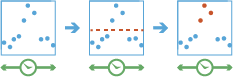

The detect_incidents task works with a time-enabled layer of points, lines, areas, or tables that represents an instant in time. Using sequentially ordered features, called tracks, this tool determines which features are incidents of interest. Incidents are determined by conditions that you specify. First, the tool determines which features belong to a track using one or more fields. Using the time at each feature, the tracks are ordered sequentially and the incident condition is applied. Features that meet the starting incident condition are marked as an incident. You can optionally apply an ending incident condition; when the end condition is ‘True’, the feature is no longer an incident. The results will be returned with the original features with new columns representing the incident name and indicate which feature meets the incident condition. You can return all original features, only the features that are incidents, or all of the features within tracks where at least one incident occurred.

For example, suppose you have GPS measurements of hurricanes every 10 minutes. Each GPS measurement records the hurricane’s name, location, time of recording, and wind speed. Using these fields, you could create an incident where any measurement with a wind speed greater than 208 km/h is an incident titled Catastrophic. By not setting an end condition, the incident would end if the feature no longer meets the start condition (wind speed slows down to less than 208).

Using another example, suppose you were monitoring concentrations of a chemical in your local water supply using a field called contanimateLevel. You know that the recommended levels are less than 0.01 mg/L, and dangerous levels are above 0.03 mg/L. To detect incidents, where a value above 0.03mg/L is an incident, and remains an incident until contamination levels are back to normal, you create an incident using a start condition of contanimateLevel > 0.03 and an end condition of contanimateLevel < 0.01. This will mark any sequence where values exceed 0.03mg/L until they return to a value less than 0.01.

Parameter	Description
input_layer	Required layer. The table, point, line or polygon features containing potential incidents. See Feature Input.
track_fields	Required string. The fields used to identify distinct tracks. There can be multiple `track_fields`.
start_condition_expression	Required string. The condition used to identify incidents. If there is no `end_condition_expression` specified, any feature that meets this condition is an incident. If there is an end condition, any feature that meets the `start_condition_expression` and does not meet the `end_condition_expression` is an incident. The expressions are Arcade expressions.
end_condition_expression	Optional string. The condition used to identify incidents. If there is no `end_condition_expression` specified, any feature that meets this condition is an incident. If there is an end condition, any feature that meets the `start_condition_expression` and does not meet the `end_condition_expression` is an incident. This is an Arcade expression.
output_mode	Optional string. Determines which features are returned. Choice list: `AllFeatures` - All of the input features are returned. `Incidents` - Only features that were found to be incidents are returned. The default value is `AllFeatures`.
time_boundary_split	Optional integer. A time boundary to detect and incident. A time boundary allows your to analyze values within a defined time span. For example, if you use a time boundary of 1 day, starting on January 1st, 1980 tracks will be analyzed 1 day at a time. The time boundary parameter was introduced in ArcGIS Enterprise 10.7. The `time_boundary_split` parameter defines the scale of the time boundary. In the case above, this would be 1. See the portal documentation for this tool to learn more.
time_split_unit	Optional string. The unit to detect an incident if time_boundary_split argument is provided. Choice list: `Milliseconds` `Seconds` `Minutes` `Hours` `Days` `Weeks` `Months` `Years`
time_reference	Optional datetime.detetime. The starting date/time where analysis will begin from.
output_name	optional string, The task will create a feature service of the results. You define the name of the service.
gis	optional `GIS` on which this tool runs. If not specified, the active GIS is used.
context	Optional dict. The context parameter contains additional settings that affect task execution. For this task, there are four settings: `extent` - A bounding box that defines the analysis area. Only those features that intersect the bounding box will be analyzed. `processSR` - The features will be projected into this coordinate system for analysis. `outSR` - The features will be projected into this coordinate system after the analysis to be saved. The output spatial reference for the spatiotemporal big data store is always WGS84. `dataStore` - Results will be saved to the specified data store. For ArcGIS Enterprise, the default is the spatiotemporal big data store.
future	Optional boolean. If `True`, a future object will be returned and the process will not wait for the task to complete. The default is `False`, which means wait for results.

Returns: FeatureLayerCollection.

# Usage Example: This example finds when and where snowplows were moving slower than 10 miles per hour by calculating the mean of a moving window of five speed values.

arcgis.env.verbose = True # set environment
arcgis.env.defaultAggregations = True # set environment

delay_incidents = output = detect_incidents(input_layer=snowplows,
                                            track_fields="plowID, dayOfYear",
                                            start_condition_expression="Mean($track.field["speed"].window(-5, 0)) < 10",
                                            output_name="Slow_Plow_Incidents")

find_dwell_locations¶

arcgis.geoanalytics.find_locations.find_dwell_locations(input_layer, track_fields, distance_tolerance, distance_unit, time_tolerance, time_unit, summary_fields=None, method='Planar', dwell_type='DwellMeanCenters', output_name=None, gis=None, context=None, future=False, time_boundary_split=None, time_boundary_unit=None, time_boundary_ref=None)¶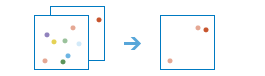

The find_dwell_locations works with time-enabled points of type instant to find where points dwell within a specific distance and duration.

Dwell locations are determined using both time (time_tolerance) and distance (distance_tolerance) values. First, the tool assigns features to a track using a unique identifier. Track order is determined by the time of features. Next, the distance between the first observation in a track and the next is calculated. Features are considered to be part of a dwell if two temporally consecutive points stay within the given distance for at least the given duration. When two features are found to be part of a dwell, the first feature in the dwell is used as a reference point, and the tool finds consecutive features that are within the specified distance of the reference point in the dwell. Once all features within the specified distance are found, the tool collects the dwell features and calculates their mean center. Features before and after the current dwell are added to the dwell if they are within the given distance of the dwell location’s mean center. This process continues until the end of the track.

For example, ecologists and conservation workers can use the Find Dwell Locations tool to improve the safety of elk during migratory seasons. Leverage the results to implement or improve protected areas in locations where the animals are spending the most time.

For another example, let’s say you work with the Department of Transportation and you want to improve traffic congestion on highways near exits. Using the Find Dwell Locations tool, you can isolate areas experiencing congestion by identifying vehicle tracks that stay within a certain distance for a certain amount of time.

Parameter	Description
input_layer	Required layer. A time-enabled layer with point features from which dwell locations will be found.
track_fields	Required String. The fields used to identify distinct tracks.
distance_tolerance	Required Float. The dwell distance tolerance is the maximum distance between points to be considered in a single dwell location. Dwell locations are determined using both distance and time.
distance_unit	Required String. The unit value.
time_tolerance	Required Integer. The dwell time tolerance is the minimum time duration of a dwell to be considered in a single dwell location. Dwell locations are determined using both distance and time.
time_unit	Required String. The time units.
summary_fields	Optional List. A list of field names and statistical summary types you want to calculate. Note that the count of points in a dwell is always returned. By default, all statistics are returned if the dwell_type specified is DwellMeanCenters (this is the default) or DwellConvexHulls. Only the count is returned if the dwell_type specified is DwellFeatures or AllFeatures. onStatisticField specifies the name of the fields in the target layer. statisticType is one of the following: `Count` - For numeric fields, this totals the number of values for all the points in each dwell. For string fields, this totals the number of strings for all the points in each dwell. `Sum` - Adds the total value of all the points in each dwell. For numeric fields. ``Mean ``- Calculates the average of all the points in each dwell. For numeric fields. `Max` - Calculates the largest value of all the points in each dwell. For numeric fields. `Range` - Finds the difference between the Min and Max values. For numeric fields. `Stddev` - Finds the standard deviation of all the points in each dwell. For numeric fields. `Var` - Finds the variance of all the points in each dwell. For numeric fields. `Any` - Returns a sample string of a point in each dwell. For string and numeric fields. `First` - Returns a the first value of a specified field in the summarized track. For string and numeric fields. This parameters was introduced at ArcGIS Enterprise 10.8.1. `Last` - Returns a the last value of a specified field in the summarized track. For string and numeric fields. This parameters was introduced at ArcGIS Enterprise 10.8.1. Example syntax for an argument: >>> summary_fields = [{"statisticType": "Mean", "onStatisticField": "Annual_Sales"}, {"statisticType": "Sum", "onStatisticField": "Annual_Sales"}]
dwell_type	Optional String. Determines which features are returned and the format. Four types are available: `DwellMeanCenters` - A point representing the centroid of each discovered dwell location. This is the default. `DwellConvexHulls` - Polygons representing the convex hull of each dwell group. `DwellFeatures` - All of the input point features determined to belong to a dwell are returned. `AllFeatures` - All of the input point features are returned.
method	Optional String. The method used to calculate distances between points. Options: `Planar` - joins points using a planar method and will not cross the international date line. This method is appropriate for local analysis on projected data. This is the default. `Geodesic` - joins points geodesically and will allow tracks to cross the international date line. This method is appropriate for large areas and geographic coordinate systems.
output_name	Optional string. The task will create a feature service of the results. You define the name of the service.
gis	Optional `GIS` on which this tool runs. If not specified, the active GIS is used.
context	Optional dict. The context parameter contains additional settings that affect task execution. For this task, there are four settings: `extent` - A bounding box that defines the analysis area. Only those features that intersect the bounding box will be analyzed. `processSR` - The features will be projected into this coordinate system for analysis. `outSR` - The features will be projected into this coordinate system after the analysis to be saved. The output spatial reference for the spatiotemporal big data store is always WGS84. `dataStore` - Results will be saved to the specified data store. For ArcGIS Enterprise, the default is the spatiotemporal big data store.
future	Optional boolean. If `True`, a future object will be returned and the process will not wait for the task to complete. The default is `False`, which means wait for results.
time_boundary_split	Optional integer. A time boundary to detect an incident. A time boundary allows you to analyze values within a defined time span. For example, if you use a time boundary of 1 day, starting on January 1st, 1980 tracks will be analyzed 1 day at a time. The time boundary parameter was introduced in ArcGIS Enterprise 10.8.1. The `time_boundary_split` parameter defines the scale of the time boundary. In the case above, this would be 1. See Find Dwell Locations <https://enterprise.arcgis.com/en/portal/latest/use/geoanalytics-find-dwell-locations.htm>_ to learn more.
time_boundary_unit	Optional string. The unit to detect an incident is time_boundary_split is used. This was introduced in ArcGIS Enterprise 10.8.1. Choice list: `Years` `Months` `Weeks` `Days` `Hours` `Minutes` `Seconds`
time_boundary_ref	Optional datetime.detetime. The starting date/time where analysis will begin from. This parameter was introduced in ArcGIS Enterprise 10.8.1.

Returns

if future is False, an output service
if future is True, a GAJob

find_similar_locations¶

arcgis.geoanalytics.find_locations.find_similar_locations(input_layer, search_layer, analysis_fields, most_or_least_similar='MostSimilar', match_method='AttributeValues', number_of_results=10, append_fields=None, output_name=None, gis=None, context=None, future=False, return_tuple=False)¶

The find_similar_locations task measures the similarity of candidate locations to one or more reference locations.

Based on criteria you specify, find_similar_locations can answer questions such as the following:

Which of your stores are most similar to your top performers with regard to customer profiles?

Based on characteristics of villages hardest hit by the disease, which other villages are high risk?

To answer questions such as these, you provide the reference locations (the input_layer parameter), the candidate locations (the search_layer parameter), and the fields representing the criteria you want to match. For example, the input_layer might be a layer containing your top performing stores or the villages hardest hit by the disease. The search_layer contains your candidate locations to search. This might be all of your stores or all other villages. Finally, you supply a list of fields to use for measuring similarity. The find_similar_locations task will rank all of the candidate locations by how closely they match your reference locations across all of the fields you have selected.

Parameter	Description
input_layer	Required layer. The `input_layer` contains one or more reference locations against which features in the `search_layer` will be evaluated for similarity. For example, the `input_layer` might contain your top performing stores or the villages hardest hit by a disease. See Feature Input. It is not uncommon for `input_layer` and `search_layer` to be the same feature service. For example, the feature service contains locations of all stores, one of which is your top performing store. If you want to rank the remaining stores from most to least similar to your top performing store, you can provide a filter for both `input_layer` and `search_layer`. The filter on `input_layer` would select the top performing store, while the filter on `search_layer` would select all stores except for the top performing store. You can use the optional filter parameter to specify reference locations. If there is more than one reference location, similarity will be based on averages for the fields you specify in the `analysis_fields` parameter. For example, if there are two reference locations and you are interested in matching population, the task will look for candidate locations in `search_layer` with populations that are most like the average population for both reference locations. If the values for the reference locations are 100 and 102, for example, the task will look for candidate locations with populations near 101. Consequently, you will want to use fields for the reference locations fields that have similar values. If, for example, the population values for one reference location is 100 and the other is 100,000, the tool will look for candidate locations with population values near the average of those two values: 50,050. Notice that this averaged value is nothing like the population for either of the reference locations.
search_layer	Required layer. The layer containing candidate locations that will be evaluated against the reference locations. See Feature Input.
analysis_fields	Required string. A list of fields whose values are used to determine similarity. They must be numeric fields, and the fields must exist on both the `input_layer` and the `search_layer`. Depending on the `match_method` selected, the task will find features that are most similar based on values or profiles of the fields.
most_or_least_similar	Optional string. The features you want to be returned. You can search for features that are either most similar or least similar to the `input_layer`, or search both the most and least similar. Choice list: `MostSimilar` `LeastSimilar` `Both` The default value is `MostSimilar`.
match_method	Optional string. The method you select determines how matching is determined. Choice list: `AttributeValues` - uses the squared differences of standardized values. `AttributeProfiles` - uses cosine similarity mathematics to compare the profile of standardized values. Using `AttributeProfiles` requires the use of at least two analysis fields. The default value is `AttributeValues`.
number_of_results	Optional integer. The number of ranked candidate locations output to `similar_result_layer`. If `number_of_results` is not set, the 10 locations will be returned. The maximum number of results is 10000. The default value is 10.
append_fields	Optional string. Optionally add fields to your data from your search layer. By default, all fields from the search layer are appended.
output_name	Optional string. The task will create a feature service of the results. You define the name of the service.
gis	Optional `GIS` on which this tool runs. If not specified, the active GIS is used.
context	Optional dict. The context parameter contains additional settings that affect task execution. For this task, there are four settings: `extent` - A bounding box that defines the analysis area. Only those features that intersect the bounding box will be analyzed. `processSR` - The features will be projected into this coordinate system for analysis. `outSR` - The features will be projected into this coordinate system after the analysis to be saved. The output spatial reference for the spatiotemporal big data store is always WGS84. `dataStore` - Results will be saved to the specified data store. For ArcGIS Enterprise, the default is the spatiotemporal big data store.
future	Optional boolean. If `True`, a future object will be returned and the process will not wait for the task to complete. The default is `False`, which means wait for results.
return_tuple	Optional boolean. If `True`, a named tuple with multiple output keys is returned. The default value is `False`.

Returns

If return_tuple is True, named tuple with the following keys:
- output: FeatureLayer
- process_info: list
if return_tuple is ``False`, a FeatureLayer

# Usage Example: To find potential retail locations based on the current top locations and their attributes.

similar_location_result = find_similar_locations(input_layer=stores_layer,
                                                 search_layer=locations,
                                                 analysis_fields="median_income, population, nearest_competitor",
                                                 most_or_least_similar="MostSimilar",
                                                 match_method="AttributeValues",
                                                 number_of_results=50,
                                                 output_name="similar_locations")

geocode_locations¶

arcgis.geoanalytics.find_locations.geocode_locations(input_layer, country=None, category=None, include_attributes=True, locator_parameters=None, output_name=None, geocode_service=None, geocode_parameters=None, gis=None, context=None, future=False)¶

The geocode_locations task geocodes a table from a big data file share. The task uses a geocode utility service configured with your portal. If you do not have a geocode utility service configured, talk to your administrator. Learn more about configuring a locator service.

When preparing to use the Geocode Location task be sure to review Best Practices for geocoding with GeoAnalytics Server.

Parameter	Description
input_layer	Required layer. The tabular input that will be geocoded. See Feature Input.
country	Optional string. If all your data is in one country, this helps improve performance for locators that accept that variable.
category	Optional string. Enter a category for more precise geocoding results, if applicable. Some geocoding services do not support category, and the available options depend on your geocode service.
include_attributes	Optional boolean. A Boolean value to return the output fields from the geocoding service in the results. To output all available output fields, set this value to ‘True’. Setting the value to false will return your original data and with geocode coordinates. Some geocoding services do not support output fields, and the available options depend on your geocode service.
locator_parameters	Optional dict. Additional parameters specific to your locator.
output_name	Optional string. The task will create a feature service of the results. You define the name of the service.
geocode_service	Optional string or Geocoder. The URL of the geocode service that you want to geocode your addresses against. The URL must end in geocodeServer and allow batch requests. The geocode service must be configured to allow for batch geocoding. For more information, see Configuring batch geocoding
geocode_parameters	optional dict. This includes parameters that help parse the input data, as well the field lengths and a field mapping. This value is the output from the AnalyzeGeocodeInput tool available on your server designated to geocode. It is important to inspect the field mapping closely and adjust them accordingly before submitting your job, otherwise your geocoding results may not be accurate. It is recommended to use the output from AnalyzeGeocodeInput and modify the field mapping instead of constructing this JSON by hand. Values: `field_info` - A list of triples with the field names of your input data, the field type (usually TEXT), and the allowed length (usually 255) `header_row_exists` - Enter `True` or `False`. `column_names` - Submit the column names of your data if your data does not have a header row `field_mapping` - Field mapping between each input field and candidate fields on the geocoding service # Example >>> geocode_parameters = {field_info: [['ObjectID', 'TEXT', 255], ['Address', 'TEXT', 255], ['Region', 'TEXT', 255], ['Postal', 'TEXT', 255]], header_row_exists - True, field_mapping: [['ObjectID', 'OBJECTID'], ['Address', 'Address'], ['Region', 'Region'], ['Postal', 'Postal']] }
gis	Optional GIS. The GIS on which this tool runs. If not specified, the active GIS is used.
context	Optional dict. Context contains additional settings that affect task execution. For this task, there are three settings: `processSR` - The features will be projected into this coordinate system for analysis. `outSR` - The features will be projected into this coordinate system after the analysis to be saved. The output spatial reference for the spatiotemporal big data store is always WGS84. `dataStore` - Results will be saved to the specified data store. For ArcGIS Enterprise, the default is the spatiotemporal big data store.
future	Optional boolean. If `True`, a future object will be returned and the process will not wait for the task to complete. The default is `False`, which means wait for results.

Returns: FeatureLayer

# Usage Example: To geocode a big data file share of mailing addresses in the United States Northwest.

geocode_server = "https://mymachine.domain.com/server/rest/services/USALocator/GeocodeServer"
geo_parameters = {"field_info": "[('ObjectID', 'TEXT', 255), ('Street', 'TEXT', 255), ('City', 'TEXT', 255), ('Region', 'TEXT', 255), ('State', 'TEXT', 255)]", "column_names": "", "file_type": "table", "header_row_exists": "true", "field_mapping": "[["Street", "Street"], ["City", "City"], ["State", "State"], ["ZIP", "ZIP"]]"}
geocode_result = find_locations.geocode_locations(input_layer=NW_addresses,
                                            output_name="geocoded_NW_USA",
                                            geocode_service=geocode_server,
                                            geocode_parameters = geo_parameters)

snap_tracks¶

arcgis.geoanalytics.find_locations.snap_tracks(point_layer, polyline_layer, track_fields, connectivity_field_matching, search_distance, search_distance_unit, distance_method='Planar', output_mode='AllFeatures', polyline_fields_to_include=None, direction_field_matching=None, output_name=None, context=None, gis=None, future=False, time_split=None, time_split_unit=None, distance_split=None, distance_split_unit=None, time_boundary_split=None, time_boundary_unit=None, time_boundary_reference=None)¶

The snap_tracks method matches track points to polylines.

Parameter	Description
point_layer	Required layer. The track point features that will be matched to polylines. See Feature Input.
polyline_layer	Required layer. The polyline features to which track points will be matched. See Feature Input.
track_fields	Required string. The fields used to identify distinct tracks. There can be multiple `track_fields`.
connectivity_field_matching	Required Dict[str,Any]. The polyline layer fields that will be used to define the connectivity of the input polyline features. The following values are required: `polylineID` - The unique identifier for the line `fromNodeID` - The node where the travel along a line is moving away from `toNodeID` - The node where the travel along a line is moving to
search_distance	Required float. The maximum distance allowed between a point and any polyline in order to be considered a match. It is recommended to use values less than or equal to 50 meters. Larger distances will result in a longer process time and less accurate results.
search_distance_unit	Required String. The unit of the search_distance.
distance_method	Optional String. The method used to calculate search distances between points and lines. Options: `Planar` - Calculates distances using a plane method and will not cross the anti-meridian. `Geodesic` - Calculates distances geodesically and will allow tracks to cross the anti-meridian. This method is appropriate for large areas and any geographic coordinate system. The default is `Planar`.
output_mode	Optional string. Determines which features are returned. Choice list: `AllFeatures` - All of the input features are returned. `Incidents` - Only features that were found to be incidents are returned. The default value is `AllFeatures`.
polyline_fields_to_include	Optional String. One or more fields from the polyine layer that will be included in the output result.
direction_field_matching	Optional dict[str, Any]. The polyline layer field and attribute values that will be used to define the direction of the input polyline features.
output_name	Optional string, The task will create a feature service of the results. You define the name of the service.
gis	Optional `GIS` on which this tool runs. If not specified, the active GIS is used.
context	Optional dict. The context parameter contains additional settings that affect task execution. For this task, there are four settings: `extent` - A bounding box that defines the analysis area. Only those features that intersect the bounding box will be analyzed. `processSR` - The features will be projected into this coordinate system for analysis. `outSR` - The features will be projected into this coordinate system after the analysis to be saved. The output spatial reference for the spatiotemporal big data store is always WGS84. `dataStore` - Results will be saved to the specified data store. For ArcGIS Enterprise, the default is the spatiotemporal big data store.
future	Optional boolean. If `True`, a GPJob is returned instead of results. The GPJob can be queried on the status of the execution. The default value is `False`.
time_split	Optional[Union[int, float]]. A time duration used to split tracks. Any features in the point_layer that are in the same track and are farther apart than this time will be split into a new track. The units of the distance values are supplied by the time_split_unit parameter.
time_split_unit	Optional[str]. The temporal unit to be used with the temporal distance value specified in time_split. Values: Milliseconds \| Seconds \| Minutes \| Hours \| Days \| Weeks\| Months \| Years
distance_split	Optional[Union[int, float]]. A distance used to split tracks.
distance_split_unit	Optional[str]. The distance unit to be used with the distance value specified in distance_split. Values: Meters \| Kilometers \| Feet \| Miles \| NauticalMiles \| Yards
time_boundary_split	Optional[int]. A time boundary allows you to analyze values within a defined time span. For example, if you use a time boundary of 1 day, starting on January 1, 1980, tracks will be analyzed one day at a time.
time_boundary_unit	Optional[str]. The unit applied to the time boundary. Values: Milliseconds \| Seconds \| Minutes \| Hours \| Days \| Weeks\| Months \| Years
time_boundary_reference	Optional[int]. A date that specifies the reference time to align the time boundary to, represented in milliseconds from epoch. The default is January 1, 1970, at 12:00 a.m. (epoch time stamp 0).

ArcGIS API for PythonAPI Reference

arcgis.geoanalytics.find_locations module

Was this page helpful?