The arcgis.geoanalytics.analyze_patterns submodule contains functions that help you identify, quantify, and visualize spatial patterns in your data.
This toolset uses distributed processing to complete analytics on your GeoAnalytics Server.
Tool |
Description |
|---|---|
calculate_density |
Calculates a magnitude-per-unit area from point features that fall within a neighborhood around each cell. |
create_space_time_cube |
Summarizes a set of points into a netCDF data structure by aggregating them into space-time bins. Within each bin, the points are counted, and specified attributes are aggregated. For all bin locations, the trend for counts and summary field values are evaluated. |
find_hot_spots |
Given a set of features, identifies statistically significant hot spots and cold spots using the Getis-Ord Gi* statistic. |
forest |
Creates models and generates predictions using an adaptation of Leo Breiman's random forest algorithm, which is a supervised machine learning method. Predictions can be performed for both categorical variables (classification) and continuous variables (regression). Explanatory variables can take the form of fields in the attribute table of the training features. In addition to validation of model performance based on the training data, predictions can be made to features. |
glr |
Performs generalized linear regression (GLR) to generate predictions or to model a dependent variable in terms of its relationship to a set of explanatory variables. This tool can be used to fit continuous (OLS), binary (logistic), and count (Poisson) models. |
gwr |
Performs Geographically Weighted Regression (GWR), which is a local form of linear regression that is used to model spatially varying relationships. |
Note: The purpose of the notebook is to show examples of the different tools that can be run on an example dataset.
Necessary imports
# connect to Enterprise GIS
from arcgis.gis import GIS
import arcgis.geoanalytics

portal_gis = GIS("your_enterprise_profile")
Adding a big data file share to the Geoanalytics server adds a corresponding big data file share item in the portal. We can search for these items using the item_type parameter.
Get the data
search_result1 = portal_gis.content.get('449e9eae6ea34fb5a3bab07463366d0a')
search_result1
data_layer = search_result1.layers[0]search_result2 = portal_gis.content.search("bigDataFileShares_ServiceCallsOrleans",
item_type = "big data file share",
max_items=40)
search_result2[<Item title:"bigDataFileShares_ServiceCallsOrleans" type:Big Data File Share owner:portaladmin>]
data_item= search_result2[0]
data_item
Querying the layers property of the item returns a feature layer representing the data.
#displays layers in the item
data_item.layers
[<Layer url:"https://pythonapi.playground.esri.com/ga/rest/services/DataStoreCatalogs/bigDataFileShares_ServiceCallsOrleans/BigDataCatalogServer/yearly_calls">]
calls = data_item.layers[0] #select first layer
calls
<Layer url:"https://pythonapi.playground.esri.com/ga/rest/services/DataStoreCatalogs/bigDataFileShares_ServiceCallsOrleans/BigDataCatalogServer/yearly_calls">
calls.properties{
"dataStoreID": "cff51a1a-4f27-4955-a3ef-5fa23240ccf9",
"fields": [
{
"name": "NOPD_Item",
"type": "esriFieldTypeString"
},
{
"name": "Type_",
"type": "esriFieldTypeString"
},
{
"name": "TypeText",
"type": "esriFieldTypeString"
},
{
"name": "Priority",
"type": "esriFieldTypeString"
},
{
"name": "MapX",
"type": "esriFieldTypeDouble"
},
{
"name": "MapY",
"type": "esriFieldTypeDouble"
},
{
"name": "TimeCreate",
"type": "esriFieldTypeString"
},
{
"name": "TimeDispatch",
"type": "esriFieldTypeString"
},
{
"name": "TimeArrive",
"type": "esriFieldTypeString"
},
{
"name": "TimeClosed",
"type": "esriFieldTypeString"
},
{
"name": "Disposition",
"type": "esriFieldTypeString"
},
{
"name": "DispositionText",
"type": "esriFieldTypeString"
},
{
"name": "BLOCK_ADDRESS",
"type": "esriFieldTypeString"
},
{
"name": "Zip",
"type": "esriFieldTypeInteger"
},
{
"name": "PoliceDistrict",
"type": "esriFieldTypeInteger"
},
{
"name": "Location",
"type": "esriFieldTypeString"
}
],
"name": "yearly_calls",
"geometryType": "esriGeometryPoint",
"type": "featureClass",
"spatialReference": {
"wkid": 102682,
"latestWkid": 3452
},
"geometry": {
"fields": [
{
"name": "MapX",
"formats": [
"x"
]
},
{
"name": "MapY",
"formats": [
"y"
]
}
]
},
"time": {
"timeType": "instant",
"timeReference": {
"timeZone": "UTC"
},
"fields": [
{
"name": "TimeCreate",
"formats": [
"MM/dd/yyyy hh:mm:ss a"
]
}
]
},
"currentVersion": 10.81,
"children": []
}Calculate Density
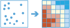
The calculate_density tool uses input point features to calculate a density map within an area of interest.
The calculate_density tool creates a density map from point features by spreading known quantities of some phenomenon (represented as attributes of the points) across the map. The result is a layer of areas classified from least dense to most dense.
For the points input, each point should represent the location of some event or incident, and the result layer will represent a count of those events or incidents per unit area. A higher density value in a new location means that there are more points near that location. In many cases, the results layer can be interpreted as a risk surface for future events. For example, if the input points represent locations of lightning strikes, the results layer can be interpreted as a risk surface for future lightning strikes.
from arcgis.geoanalytics.analyze_patterns import calculate_density
from datetime import datetime as dt
This example calculates the density of calls using 1-Meter bins and a 100-Meter neighborhood. The results layer will show areas with high and low call counts, and this information can be used by police departments to better allocate resources to high crime areas.
##usage example
cal_density = calculate_density(calls,
                                weight='Uniform',
                                bin_type='Square',
                                bin_size=1,
                                bin_size_unit="Kilometers",
                                time_step_interval=1,
                                time_step_interval_unit="Years",
                                time_step_repeat_interval=1,
                                time_step_repeat_interval_unit="Months",
                                time_step_reference=dt(2011, 1, 1),
                                radius=1000,
                                radius_unit="Meters",
                                area_units='SquareKilometers',
                                output_name="calculate density of call" + str(dt.now().microsecond))
cal_density
{"messageCode":"BD_101051","message":"Possible issues were found while reading 'inputLayer'.","params":{"paramName":"inputLayer"}}
{"messageCode":"BD_101052","message":"Some records have either missing or invalid time values."}
{"messageCode":"BD_101054","message":"Some records have either missing or invalid geometries."}


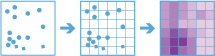
Create Space Time Cube
The Create Space Time Cube tool summarizes a set of points into a netCDF data structure by aggregating them into space-time bins. Within each bin, the points are counted and their specified attributes are aggregated. For all bin locations, the trend for counts and summary field values are evaluated.
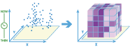
The create_space_time_cube tool works with a layer of point features that are time enabled. It aggregates the data into a three-dimensional cube of space-time bins. When determining the point in a space-time bin relationship, statistics about all points in the space-time bins are calculated and assigned to the bins. The most basic statistic is the number of points within the bins, but you can calculate other statistics as well. For example, suppose you have point features of crimes in a city and you want to summarize the number of crimes in both space and time. You can calculate the space-time cube for the dataset and use the cube to further analyze trends, such as emerging hot and cold spots.
from arcgis.geoanalytics.analyze_patterns import create_space_time_cubeThis example creates a space time cube of cells using 5-Mile bins and a 1-day time step.
##usage example
create_space_time_cube(point_layer=calls,
                       bin_size=100,
                       bin_size_unit="Miles",
                       time_step_interval=1,
                       time_step_interval_unit="Days",
                       time_step_alignment='StartTime',
                       output_name="space_time_cube")
Attaching log redirect Log level set to DEBUG Detaching log redirect
{"url": "https://pythonapi.playground.esri.com/ga/rest/directories/arcgisjobs/system/geoanalyticstools_gpserver/j2c39be7b2a8a490b95df1383cdc355e6/scratch/space_time_cube.nc"}As you open the link in your browser, you will notice a .nc file will begin to download. With this file, you can now visualize the space time cube in ArcGIS Pro.

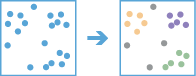
Find Hot Spots
The find_hot_spots tool determines if there is any statistically significant clustering in the spatial pattern of your data.
The find_hot_spots tool analyzes point data (such as crime incidents, traffic accidents, trees, and so on) or field values associated with points. It finds statistically significant spatial clusters of high incidents (hot spots) and low incidents (cold spots). Hot spots are locations with lots of points and cold spots are locations with very few points.
The result map layer shows hot spots in red and cold spots in blue. The darkest red features indicate the strongest clustering of point densities; you can be 99 percent confident that the clustering associated with these features could not be the result of random chance. Similarly, the darkest blue features are associated with the strongest spatial clustering of the lowest point densities. Features that are beige are not part of a statistically significant cluster; the spatial pattern associated with these features could very likely be the result of random processes and random chance.
from arcgis.geoanalytics.analyze_patterns import find_hot_spots
from datetime import datetime as dt
This example finds hot spots of calls with a hot spot cell size of 100 Meters.
##usage example
hot_spots = find_hot_spots(calls,
                           bin_size=100,
                           bin_size_unit='Meters',
                           neighborhood_distance=250,
                           neighborhood_distance_unit='Meters',
                           output_name="get hot spot areas" + str(dt.now().microsecond))
hot_spots
Find Point Clusters
The find_point_clusters tool finds clusters of point features in surrounding noise based on their spatial or spatiotemporal distribution.
This tool extracts clusters from your input point features and identifies any surrounding noise.
For example, a nongovernmental organization could be studying a particular pest-borne disease. It has a point dataset representing households in a study area, some of which are infested, and some of which are not. By using the Find Point Clusters tool, an analyst can determine clusters of infested households to help pinpoint an area to begin treatment and extermination of the pests.
from arcgis.geoanalytics.analyze_patterns import find_point_clustersThis example finds clusters of calls within a 1 mile search distance, forming clusters specified by the min_feature_clusters parameter. min_feature_clusters is the number of features that must be found within a search range of a point for that point to start forming a cluster.
##usage example
point_clusters = find_point_clusters(calls_sample,
                                     method='HDBSCAN',
                                     min_feature_clusters=5,
                                     output_name='point clusters' + str(dt.now().microsecond))
{"messageCode":"BD_101051","message":"Possible issues were found while reading 'inputLayer'.","params":{"paramName":"inputLayer"}}
{"messageCode":"BD_101052","message":"Some records have either missing or invalid time values."}
{"messageCode":"BD_101054","message":"Some records have either missing or invalid geometries."}
point_clusters
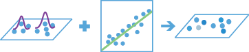
Forest
The forest method creates models and generates predictions using an adaptation of Leo Breiman's random forest algorithm, which is a supervised machine learning method. Predictions can be performed for both categorical variables (classification) and continuous variables (regression). Explanatory variables can take the form of fields in the attribute table of the training features. In addition to validation of model performance based on the training data, predictions can be made into features.

from arcgis.geoanalytics.analyze_patterns import forestThis example predicts total solar energy produced using variables like the following:
- wind_speed : wind speed(m/sec)
- dayl_s : Day length (sec/day)
- prcp__mm_d : Precipitation (mm/day)
- srad_W_m : Shortwave radiation (W/m^2)
- swe_kg_m : Snow water equivalent (kg/m^2)
- tmax__deg : Maximum air temperature (degrees C)
- tmin__deg : Minimum air temperature (degrees C)
- vp_Pa : Water vapor pressure (Pa)
For more details, refer here
##usage example
forest(input_layer=data_layer,
       var_prediction={"fieldName":"capacity_f", "categorical":False},
       var_explanatory=[{"fieldName":"altitude_m", "categorical":False},
                        {"fieldName":"wind_speed", "categorical":False},
                        {"fieldName":"dayl__s_", "categorical":False},
                        {"fieldName":"prcp__mm_d", "categorical":False},
                        {"fieldName":"srad__W_m_", "categorical":False},
                        {"fieldName":"swe__kg_m_", "categorical":False},
                        {"fieldName":"tmax__deg", "categorical":False},
                        {"fieldName":"tmin__deg", "categorical":False},
                        {"fieldName":"vp__Pa_", "categorical":False}
                       ],
       prediction_type="TrainAndPredict",
       trees=200,
importance_tbl=True)GLR
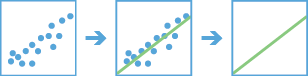
Generalized Linear Regression (GLR) performs a Generalized Linear Regression to generate predictions or model a dependent variable in terms of its relationship to a set of explanatory variables. This tool can be used to fit continuous (Gaussian), binary (logistic), and count (Poisson) models.
from arcgis.geoanalytics.analyze_patterns import glrglr_output = glr(data_layer,
var_dependent='capacity_f',
var_explanatory=['altitude_m', 'wind_speed', 'dayl__s_', 'prcp__mm_d',
'srad__W_m_','swe__kg_m_','tmax__deg','tmin__deg','vp__Pa_'],
output_name='glr' + str(dt.now().microsecond))
glr_outputGWR
The GWR tool performs a Geographically Weighted Regression, which is a local form of linear regression used to model spatially varying relationships.
The following are examples of the types of questions you can answer using this tool:
- Is the relationship between educational attainment and income consistent across the study area?
- What are the key variables that explain high forest fire frequency?
- Where are the districts in which children are achieving high test scores? What characteristics seem to be associated? Where is each characteristic most important?
from arcgis.geoanalytics.analyze_patterns import gwr#get new data
gwr_output = gwr(hurricanes,
dependent_variable=['season'],
explanatory_variables=['wind', 'wind_wmo1', 'pres_wmo_'],
number_of_neighbors=100,
output_name='gwr' + str(dt.now().microsecond))
gwr_output{"messageCode":"BD_101255","message":"Unable to estimate at least one local model due to multicollinearity."}
{"messageCode":"BD_101256","message":"Unable to predict the dependent variable value for one or more features."}
{"messageCode":"BD_101051","message":"Possible issues were found while reading 'inputLayer'.","params":{"paramName":"inputLayer"}}
{"messageCode":"BD_101052","message":"Some records have either missing or invalid time values."}
In this guide, we learned about tools that help to identify, quantify, and visualize patterns in data. In the next guide, we will learn about tools that help in finding desired locations based on a criteria.