The arcgis.geoanalytics.summarize_data submodule contains functions that calculate total counts, lengths, areas, and basic descriptive statistics of features and their attributes within areas or near other features.
This toolset uses distributed processing to complete analytics on your GeoAnalytics Server.
Tool |
Description |
|---|---|
aggregate_points |
Aggregates points into polygon features or bins. A polygon is returned with a count of points as well as optional statistics at all locations where points exist. |
build_multivariable_grid |
Generates a grid of square or hexagonal bins and calculates variables for each bin based on the proximity of one or more input layers. |
describe_dataset |
Summarizes features into calculated field statistics, sample features, and extent boundaries. |
join_features |
Joins attributes from one layer to another based on spatial, temporal, or attribute relationships, or a combination of those relationships. |
reconstruct_tracks |
Creates line or polygon tracks from time-enabled input data. |
summarize_attributes |
Calculates summary statistics for fields in a feature class. |
summarize_center_and_dispersion |
Finds central features and directional distributions and calculates mean and median locations from the input. |
summarize_within |
Overlays a polygon layer with another layer to summarize the number of points, length of the lines, or area of the polygons within each polygon and calculates attribute field statistics about those features within the polygons. |
Note: The purpose of the notebook is to show examples of the different tools that can be run on an example dataset.
Connect to your gis
# connect to Enterprise GIS
from arcgis.gis import GIS
import arcgis.geoanalytics

portal_gis = GIS("your_enterprise_profile")
Search items registered with your server
search_result = portal_gis.content.search("bigDataFileShares_all_hurricanes", item_type = "big data file share")[0]
search_result
years_50 = search_result.layers[0]search_result = portal_gis.content.search("bigDataFileShares_all_hurricanes", item_type = "big data file share")[0]
search_resultsearch_result.layers[<Layer url:"https://pythonapi.playground.esri.com/ga/rest/services/DataStoreCatalogs/bigDataFileShares_all_hurricanes/BigDataCatalogServer/hurricanes">]
search_result.layers[<Layer url:"https://pythonapi.playground.esri.com/ga/rest/services/DataStoreCatalogs/bigDataFileShares_GA_Data/BigDataCatalogServer/air_quality">, <Layer url:"https://pythonapi.playground.esri.com/ga/rest/services/DataStoreCatalogs/bigDataFileShares_GA_Data/BigDataCatalogServer/crime">, <Layer url:"https://pythonapi.playground.esri.com/ga/rest/services/DataStoreCatalogs/bigDataFileShares_GA_Data/BigDataCatalogServer/calls">, <Layer url:"https://pythonapi.playground.esri.com/ga/rest/services/DataStoreCatalogs/bigDataFileShares_GA_Data/BigDataCatalogServer/analyze_new_york_city_taxi_data">]
search_result = portal_gis.content.search("bigDataFileShares_ServiceCallsOrleans", item_type = "big data file share")[0]
search_resultcalls = search_result.layers[0]search_result = portal_gis.content.search("bigDataFileShares_ServiceCallsOrleans", item_type = "big data file share")[0]
search_resultcalls = search_result.layers[0]calls = search_result[0].layers[2]
hurricanes = search_result.lyers[1]search_result = portal_gis.content.search("bigDataFileShares_Chicago_Crimes", item_type = "big data file share")
search_result[<Item title:"bigDataFileShares_Chicago_Crimes_2" type:Big Data File Share owner:admin>, <Item title:"bigDataFileShares_Chicago_Crimes" type:Big Data File Share owner:admin>]
homicides = portal_gis.content.get('79a9c31548cb4de2a17b06a9e67095ba')blk_grp = portal_gis.content.get('eb37f3fb4d854040b8ae7a74323299e5')crimes_lyr = search_result[1].layers[0]
homicides_lyr = homicides.layers[0]
blk_grp_lyr = blk_grp.layers[0]Aggregate Points
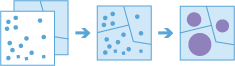
This aggregate_points tool works with a layer of point features and a layer of areas. The layer of areas can be an input polygon layer or it can be square or hexagonal bins calculated when the task is run. The tool first determines which points fall within each specified area. After determining this point-in-area spatial relationship, statistics about all points in the area are calculated and assigned to the area. The most basic statistic is the count of the number of points within the area, but you can get other statistics as well.
This tool can also work on data that is time-enabled. If time is enabled on the input points, then the time slicing options are available. Time slicing allows you to calculate the point-in area relationship while looking at a specific slice in time. For example, you could look at hourly intervals, which would result in outputs for each hour.
For an example with time, suppose you had point features of every transaction made at a coffee shop location and no area layer. The data has been recorded over a year, and each transaction has a location and a time stamp. Assuming each transaction has a TOTAL_SALES attribute, you can get the sum of all TOTAL SALES within the space and time of interest. If these transactions are for a single city, we could generate areas that are one kilometer grids, and look at weekly time slices to summarize the transactions in both time and space.
from arcgis.geoanalytics.summarize_data import aggregate_pointsagg_result = aggregate_points(orleans_calls,
polygon_layer=blk_grp_lyr,
output_name="aggregate results of call" + str(dt.now().microsecond)){"messageCode":"BD_101068","message":"Bin generation and analysis requires a projected coordinate system and a default projection of World Cylindrical Equal Area has been applied."}
{"messageCode":"BD_101054","message":"Some records have either missing or invalid geometries."}
{"messageCode":"BD_101088","message":"Some result features were clipped to the valid extent of the resulting spatial reference."}

To learn more about the aggregate_points tool, please read api-reference for help.
Build Multi-Variable Grid

The build_multivariable_grid task works with one or more layers of point, line, or polygon features. The task generates a grid of square or hexagonal bins and compiles information about each input layer into each bin. For each input layer, this information can include the following variables:
-
Distance to Nearest - The distance from each bin to the nearest feature.
-
Attribute of Nearest - An attribute value of the feature nearest to each bin.
-
Attribute Summary of Related - A statistical summary of all features within search_distance of each bin.
Only variables you specify in variable_calculations will be included in the result layer. These variables can help you understand the proximity of your data throughout the extent of your analysis. The results can help you answer questions like:
- Given multiple layers of public transportation infrastructure, what part of the city is least accessible by public transportation?
- Given layers of lakes and rivers, what is the name of the water body closest to each location in the U.S.?
- Given a layer of household income, where in the U.S. is the variation of income in the surrounding 50 miles the greatest?
The results of build_multivariable_grid can also be used in prediction and classification workflows. The task allows you to calculate and compile information from many different data sources into a single spatially continuous layer in one step. This layer can then be used with the Enrich From Multi-Variable Grid task to quickly enrich point features with the variables you have calculated, reducing the amount of effort required to build prediction and classification models from point data.
from arcgis.geoanalytics.summarize_data import build_multivariable_gridvar_calc = [{"layer":0,"variables":[{"type":"AttributeOfNearest",
"outFieldName":"test",
"attributeField":"Location",
"searchDistance":6,
"searchDistanceUnit":"Miles"}]}]This example creates a multivariable grid by summarizing information about the attributes of the nearest locations.
##usage example
output = build_multivariable_grid(input_layers=[calls],
                                  variable_calculations=var_calc,
                                  bin_size=5,
                                  bin_unit='Miles',
                                  bin_type='Square',
                                  output_name='build_multivariable_grid')
output
Describe Dataset
The describe_dataset task provides an overview of your big data. The tool outputs a feature layer representing either a sample of your input features or a single polygon feature layer that represents the extent of your input features. You can choose to output one, both, or none.
For example, imagine you are tasked with completing an analysis workflow on a large volume of data. You want to try the workflow, but it could take hours or days with your full dataset. Instead of using time and resources to run the full analysis, you can first create a sample layer to efficiently test your workflow before running it on the full dataset.
from arcgis.geoanalytics.summarize_data import describe_dataset
from datetime import datetime as dt
description = describe_dataset(input_layer=calls,
extent_output=True,
sample_size=1000,
output_name="Description of service calls" + str(dt.now().microsecond),
return_tuple=True)description.output<FeatureLayer url:"https://pythonapi.playground.esri.com/server/rest/services/Hosted/Description_of_service_calls645206/FeatureServer/0">
description.output_json{'datasetName': 'yearly_calls',
'datasetSource': 'Big Data File Share - ServiceCallsOrleans',
'recordCount': 510153,
'geometry': {'geometryType': 'Point',
'sref': {'wkid': 102682, 'latestWkid': 3452},
'countNonEmpty': 510153,
'countEmpty': 0,
'spatialExtent': {'xmin': 3659898,
'ymin': 501901,
'xmax': 37369000,
'ymax': 3513814}},
'time': {'timeType': 'Instant',
'countNonEmpty': 510153,
'countEmpty': 0,
'temporalExtent': {'start': '2011-01-01 00:00:02.000',
'end': '2011-12-31 23:57:11.000'}}}
Join Features
Using either feature layers or tabular data, you can join features and records based on specific relationships between the input layers or tables. Joins will be determined by spatial, temporal, and attribute relationships, and summary statistics can be optionally calculated.
For example:
-
Given point locations of crime incidents with a time, join the crime data to itself specifying a spatial relationship of crimes within 1 kilometer of each other and that occurred within 1 hour of each other to determine if there are a sequence of crimes close to each other in space and time.
-
Given a table of ZIP Codes with demographic information and area features representing residential buildings, join the demographic information to the residences so each residence now has the information.
The Join_features task works with two layers. join_features joins attributes from one feature to another based on spatial, temporal, or attribute relationships, or some combination of the three. The tool determines all input features that meet the specified join conditions and joins the second input layer to the first. You can optionally join all features to the matching features or summarize the matching features.
Join_features can be applied to points, lines, areas, and tables. A temporal join requires that your input data is time-enabled, and a spatial join requires that your data has a geometry.
from arcgis.geoanalytics.summarize_data import join_featuresjoin_features(target_layer=homicides_lyr,
join_layer=crimes_lyr,
join_operation='JoinOneToOne',
attribute_relationship=[{"targetField":"beat","operator":"equal","joinField":"Beat"}],
output_name='join features'){"messageCode":"BD_101051","message":"Possible issues were found while reading 'targetLayer'.","params":{"paramName":"targetLayer"}}
{"messageCode":"BD_101054","message":"Some records have either missing or invalid geometries."}
{"messageCode":"BD_101051","message":"Possible issues were found while reading 'joinLayer'.","params":{"paramName":"joinLayer"}}
{"messageCode":"BD_101054","message":"Some records have either missing or invalid geometries."}


Reconstruct Tracks
The Reconstruct Tracks tool connects time-sequential points to tracks and summarizes features within the tracks. Tracks are identified by one or more track fields. The resulting layer displays the track as a line or area, the count of the features within a track that have been summarized, and any additional statistics that have been specified.
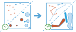
The reconstruct_tracks task works with a time-enabled layer of either point or polygon features that represents an instant in time. It first determines which features belong to a track using an identifier. Using the time at each location, the tracks are ordered sequentially and transformed into a line or polygon representing the path of movement over time. Optionally, the input can be buffered by a field, which will create a polygon at each location. These buffered points, or polygons if the inputs are polygons, are then joined sequentially to create a track as a polygon where the width is representative of the attribute of interest. Resulting tracks have start and end times that represent the time at the first and last feature in a given track. When the tracks are created, statistics about the input features are calculated and assigned to the output track. The most basic statistic is the count of points within the area, but other statistics can be calculated as well. Features in time-enabled layers can be represented in one of two ways:
-
Instant - A single moment in time
-
Interval - A start and end time
For example, suppose you have GPS measurements of hurricanes every 10 minutes. Each GPS measurement records a hurricane's name, location, time of recording, and wind speed. You could create tracks of the hurricanes using the names of the hurricanes as the track identification, and all hurricanes’ tracks would be generated. You could then calculate statistics, such as the mean, maximum, and minimum wind speed of each hurricane, as well as the count of measurements in each track.
from arcgis.geoanalytics.summarize_data import reconstruct_tracksThis example aggregates numerous points into line segments showing the tracks followed by the hurricanes. The tool creates a feature layer item as an output that can be accessed once the processing is complete.
##usage example
result = reconstruct_tracks(years_50,
                            track_fields='Serial_Num',
                            method='GEODESIC')
result
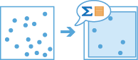
Summarize Attributes
The Summarize Attributes tool summarizes like field values to generate a summary table. The resulting layer displays the count of features that have been summarized, as well as any additional statistics that have been specified.

The summarize_attributes operation takes an input layer and summarizes and calculates statistics for like values. The most basic statistic is the count of features with a specified value, but other statistics can be calculated as well. You can also summarize values into time steps.
For example, if you have a point layer of store locations with a field representing the DISTRICT_MANAGER_NAME and you want to summarize coffee sales by manager, you can specify the DISTRICT_MANAGER_NAME field as the field to dissolve on, and all rows of data representing individual managers will be summarized. This means all store locations managed by Manager1 will be summarized into one row with summary statistics calculated. In this instance, statistics like the number of stores and the sum of TOTAL_SALES for all stores that Manager1 manages will be calculated. These would also be calculated for any other manager listed in the DISTRICT_MANAGER_NAME field.
from arcgis.geoanalytics.summarize_data import summarize_attributessummarized_features = summarize_attributes(input_layer=years_50,
fields='track_type')
summarized_features
Summarize Center and Dispersion
The summarize_center_and_dispersion task finds central features and directional distributions. It can be used to answer questions like:
- Where is the center?
- Which feature is the most accessible from all other features?
- How dispersed, compact, or integrated are the features?
- Are there directional trends?
For an example, suppose you have used the GeoAnalytics tool Find Point Clusters to identify groups of power outages across an entire year. The result will be time enabled points representing cluster locations of power outages. However, you are interested in identifying the center of the power outages for visualization. To do this, you could use Summarize Center And Dispersion to group by the outage cluster ids field.

Note: This tool is available in ArcGIS Enterprise version 10.9 and later.
from arcgis.geoanalytics.summarize_data import summarize_center_and_dispersionoutput_trends = summarize_center_and_dispersion(input_layer=years_50,
summary_type='MedianCenter',
output_name='directional trends')
output_trends
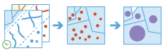
Summarize Within
The Summarize Within tool calculates statistics in areas where an input layer is within or overlapping a boundary layer. The area you are summarizing within can be an area layer or a hexagonal or square bin.
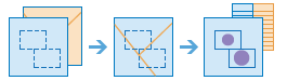
The summarize_within task finds features (and portions of features) that are within the boundaries of areas in the first input layer. Some example use cases are:
- Given a layer of watershed boundaries and a layer of land-use boundaries, calculate the total acreage of land-use type for each watershed.
- Given a layer of parcels in a county and a layer of city boundaries, summarize the average value of vacant parcels within each city boundary.
- Given a layer of counties and a layer of roads, summarize the total mileage of roads by road type within each county.
You can think of summarize_within as taking two layers and stacking them on top of each other. One of the layers, summary_polygons, must be a polygon layer, and imagine that these polygon boundaries are all colored red. The other layer, summarized_layer, can be any feature type—point, line, or polygon. After stacking these layers on top of each other, you peer down through the stack and count the number of features in summarized_layer that fall within the polygons with the red boundaries (summary_polygons). Not only can you count the number of features, you can calculate simple statistics about the attributes of the features in summarized_layer, such as sum, mean, minimum, maximum, and so on.
from arcgis.geoanalytics.summarize_data import summarize_within##usage example
summarised_features = summarize_within(years_50,
bin_type="Square",
bin_size=5,
bin_size_unit='Miles',
standard_summary_fields=[{"statisticType" : "average", "onStatisticField" : "Wind" }],
output_name='summmrized_features')
summarised_features
In this guide, we learned about tools that summarize big data. In the next guide, we will learn about tools that find proximity.