Introduction
Dashboards, statistics, and other information about the COVID-19 are floating all over the internet, and different countries or regions are adopting varied strategies, from complete lockdown, to social distancing, to herd immunity, you might be confused at what is the right strategy, and which information is valid. This notebook is not providing you a final answer, but tools or methods that you can try yourself in performing data modeling, analyzing, and predicting the spread of COVID-19 with the ArcGIS API for Python, and other libraries such as pandas and numpy. Hopefully, given the workflow demonstrations, you are able to find the basic facts, current patterns, and future trends behind the common notions about how COVID-19 spread from a dataset perspective [1,2,3,4].
Before we dive into data science and analytics, let's start with importing the necessary modules:
import pandas as pd
import numpy as np
import matplotlib.pyplot as plt
import time
from arcgis.gis import GIS
Import and Understand Source Dataset
Among all the official and unofficial data sources on the web providing COVID-19 related data, one of the most widely used dataset today is the one provided by the John Hopkins University's Center for Systems Science and Engineering (JHU CSSE), which can be accessed on GitHub under the name - Novel Coronavirus (COVID-19) Cases, provided by JHU CSSE [5,10,11,12]. The time-series consolidated data needed for all the analysis to be performed in this notebook fall into these two categories:
- Type: Confirmed Cases, Deaths, and the Recovered;
- Geography: Global, and the United States only.
Now let's first look at the U.S. dataset.
Time-series data for the United States
The dataset can be directly imported into data-frames with read_csv method in Pandas. Compared to downloading the file manually and then read it, it is preferred to use the URLs (which point to the CSV files archived on GitHub) because as situation changes, it becomes easier to load and refresh the analysis with new data.
Now, let's read the time-series data of the confirmed COVID-19 cases in the United States from the GitHub source url, into a Pandas DataFrame:
# read time-series csv
usa_ts_url = 'https://raw.githubusercontent.com/CSSEGISandData/COVID-19/master/csse_covid_19_data/csse_covid_19_time_series/time_series_covid19_confirmed_US.csv'
usa_ts_df = pd.read_csv(usa_ts_url, header=0, escapechar='\\')
usa_ts_df.head(5)| UID | iso2 | iso3 | code3 | FIPS | Admin2 | Province_State | Country_Region | Lat | Long_ | ... | 6/26/20 | 6/27/20 | 6/28/20 | 6/29/20 | 6/30/20 | 7/1/20 | 7/2/20 | 7/3/20 | 7/4/20 | 7/5/20 | |
|---|---|---|---|---|---|---|---|---|---|---|---|---|---|---|---|---|---|---|---|---|---|
| 0 | 16 | AS | ASM | 16 | 60.0 | NaN | American Samoa | US | -14.2710 | -170.1320 | ... | 0 | 0 | 0 | 0 | 0 | 0 | 0 | 0 | 0 | 0 |
| 1 | 316 | GU | GUM | 316 | 66.0 | NaN | Guam | US | 13.4443 | 144.7937 | ... | 247 | 247 | 247 | 253 | 257 | 267 | 280 | 280 | 280 | 280 |
| 2 | 580 | MP | MNP | 580 | 69.0 | NaN | Northern Mariana Islands | US | 15.0979 | 145.6739 | ... | 30 | 30 | 30 | 30 | 30 | 30 | 31 | 31 | 31 | 31 |
| 3 | 630 | PR | PRI | 630 | 72.0 | NaN | Puerto Rico | US | 18.2208 | -66.5901 | ... | 6922 | 7066 | 7189 | 7250 | 7465 | 7537 | 7608 | 7683 | 7787 | 7916 |
| 4 | 850 | VI | VIR | 850 | 78.0 | NaN | Virgin Islands | US | 18.3358 | -64.8963 | ... | 81 | 81 | 81 | 81 | 81 | 90 | 92 | 98 | 111 | 111 |
5 rows × 177 columns
usa_ts_df.columnsIndex(['UID', 'iso2', 'iso3', 'code3', 'FIPS', 'Admin2', 'Province_State',
'Country_Region', 'Lat', 'Long_',
...
'6/26/20', '6/27/20', '6/28/20', '6/29/20', '6/30/20', '7/1/20',
'7/2/20', '7/3/20', '7/4/20', '7/5/20'],
dtype='object', length=177)As we can see from the printouts of usa_ts_df.columns, the first 11 columns are displayed as ['UID', 'iso2', 'iso3', 'code3', 'FIPS', 'Admin2', 'Province_State', 'Country_Region', 'Lat', 'Long_'], while the rest of the columns are dates from 1/22/20 to the most current date on record.
date_list = usa_ts_df.columns.tolist()[11:]
date_list[0], date_list[-1]
('1/22/20', '7/5/20')Repair and Summarize the state-wide time-series data
Look at the last five rows of the DataFrame usa_ts_df, and see that they are all cases for Province_State=="Utah":
usa_ts_df.tail()| UID | iso2 | iso3 | code3 | FIPS | Admin2 | Province_State | Country_Region | Lat | Long_ | ... | 6/26/20 | 6/27/20 | 6/28/20 | 6/29/20 | 6/30/20 | 7/1/20 | 7/2/20 | 7/3/20 | 7/4/20 | 7/5/20 | |
|---|---|---|---|---|---|---|---|---|---|---|---|---|---|---|---|---|---|---|---|---|---|
| 3256 | 84070016 | US | USA | 840 | NaN | Central Utah | Utah | US | 39.372319 | -111.575868 | ... | 127 | 134 | 143 | 159 | 169 | 173 | 180 | 194 | 201 | 209 |
| 3257 | 84070017 | US | USA | 840 | NaN | Southeast Utah | Utah | US | 38.996171 | -110.701396 | ... | 33 | 34 | 35 | 35 | 36 | 37 | 39 | 40 | 40 | 40 |
| 3258 | 84070018 | US | USA | 840 | NaN | Southwest Utah | Utah | US | 37.854472 | -111.441876 | ... | 1302 | 1361 | 1428 | 1467 | 1519 | 1553 | 1584 | 1625 | 1660 | 1689 |
| 3259 | 84070019 | US | USA | 840 | NaN | TriCounty | Utah | US | 40.124915 | -109.517442 | ... | 45 | 46 | 48 | 48 | 50 | 50 | 52 | 53 | 55 | 55 |
| 3260 | 84070020 | US | USA | 840 | NaN | Weber-Morgan | Utah | US | 41.271160 | -111.914512 | ... | 814 | 846 | 872 | 919 | 954 | 1004 | 1042 | 1090 | 1172 | 1195 |
5 rows × 177 columns
Some rows in the DataFrame are of many-rows-to-one-state matching, while others are of the one-row-to-one-state matching replationship. All records listed in the usa_ts_df with Admin2 not equal to NaN, are those rows that fall into the category of "many-rows-to-one-state" matching.
usa_ts_df[usa_ts_df["Admin2"].notna()].head()| UID | iso2 | iso3 | code3 | FIPS | Admin2 | Province_State | Country_Region | Lat | Long_ | ... | 6/26/20 | 6/27/20 | 6/28/20 | 6/29/20 | 6/30/20 | 7/1/20 | 7/2/20 | 7/3/20 | 7/4/20 | 7/5/20 | |
|---|---|---|---|---|---|---|---|---|---|---|---|---|---|---|---|---|---|---|---|---|---|
| 5 | 84001001 | US | USA | 840 | 1001.0 | Autauga | Alabama | US | 32.539527 | -86.644082 | ... | 482 | 492 | 497 | 521 | 530 | 545 | 553 | 560 | 583 | 607 |
| 6 | 84001003 | US | USA | 840 | 1003.0 | Baldwin | Alabama | US | 30.727750 | -87.722071 | ... | 500 | 539 | 559 | 626 | 663 | 686 | 735 | 828 | 846 | 864 |
| 7 | 84001005 | US | USA | 840 | 1005.0 | Barbour | Alabama | US | 31.868263 | -85.387129 | ... | 309 | 314 | 314 | 319 | 322 | 323 | 333 | 345 | 347 | 349 |
| 8 | 84001007 | US | USA | 840 | 1007.0 | Bibb | Alabama | US | 32.996421 | -87.125115 | ... | 150 | 158 | 159 | 162 | 167 | 171 | 176 | 186 | 187 | 190 |
| 9 | 84001009 | US | USA | 840 | 1009.0 | Blount | Alabama | US | 33.982109 | -86.567906 | ... | 181 | 185 | 186 | 196 | 204 | 214 | 218 | 226 | 230 | 235 |
5 rows × 177 columns
As shown in the output of the previous two cells, we can see that for the usa_ts_df which we have created and parsed from the U.S. Dataset, there are multiple rows per state representing different administrative areas of the state with reported cases. Next, we will use the to-be-defined function sum_all_admins_in_state() to summarize all administrative areas in one state into a single row.
def sum_all_admins_in_state(df, state):

    # query all sub-records of the selected state
    tmp_df = df[df["Province_State"]==state]

    # create a new row which is to sum all statistics of this state, and
    # assign the summed value of all sub-records to the date_time column of the new row
    sum_row = tmp_df.sum(axis=0)

    # assign the constants to the ['Province/State', 'Country/Region', 'Lat', 'Long'] columns;
    # note that the Province/State column will be renamed from solely the country name to country name + ", Sum".
    sum_row.loc['UID'] = "NaN"
    sum_row.loc['Admin2'] = "NaN"
    sum_row.loc['FIPS'] = "NaN"
    sum_row.loc['iso2'] = "US"
    sum_row.loc['iso3'] = "USA"
    sum_row.loc['code3'] = 840
    sum_row.loc['Country_Region'] = "US"
    sum_row.loc['Province_State'] = state + ", Sum"
    sum_row.loc['Lat'] = tmp_df['Lat'].values[0]
    sum_row.loc['Long_'] = tmp_df['Long_'].values[0]

    # append the new row to the original DataFrame, and
    # remove the sub-records of the selected country.
    df = pd.concat([df, sum_row.to_frame().T], ignore_index=True)
    #display(df[df["Province_State"].str.contains(state + ", Sum")])
    df=df[df['Province_State'] != state]
    df.loc[df.Province_State == state+", Sum", 'Province_State'] = state

    return df
# loop thru all states in the U.S.
for state in usa_ts_df.Province_State.unique():
usa_ts_df = sum_all_admins_in_state(usa_ts_df, state)Now with sum_all_admins_in_state applied to all states, we shall be expecting usa_ts_df to be with all rows converted to one-row-to-one-state matching. Let's browse the last five rows in the DataFrame to validate the results.
usa_ts_df.tail()| UID | iso2 | iso3 | code3 | FIPS | Admin2 | Province_State | Country_Region | Lat | Long_ | ... | 6/26/20 | 6/27/20 | 6/28/20 | 6/29/20 | 6/30/20 | 7/1/20 | 7/2/20 | 7/3/20 | 7/4/20 | 7/5/20 | |
|---|---|---|---|---|---|---|---|---|---|---|---|---|---|---|---|---|---|---|---|---|---|
| 54 | NaN | US | USA | 840 | NaN | NaN | West Virginia | US | 39.1307 | -80.0035 | ... | 2730 | 2782 | 2832 | 2870 | 2905 | 2979 | 3053 | 3126 | 3205 | 3262 |
| 55 | NaN | US | USA | 840 | NaN | NaN | Wisconsin | US | 43.9697 | -89.7678 | ... | 26747 | 27286 | 27743 | 28058 | 28659 | 29199 | 29738 | 30317 | 31055 | 31577 |
| 56 | NaN | US | USA | 840 | NaN | NaN | Wyoming | US | 41.655 | -105.724 | ... | 1368 | 1392 | 1417 | 1450 | 1487 | 1514 | 1550 | 1582 | 1606 | 1634 |
| 57 | NaN | US | USA | 840 | NaN | NaN | Diamond Princess | US | 0 | 0 | ... | 49 | 49 | 49 | 49 | 49 | 49 | 49 | 49 | 49 | 49 |
| 58 | NaN | US | USA | 840 | NaN | NaN | Grand Princess | US | 0 | 0 | ... | 103 | 103 | 103 | 103 | 103 | 103 | 103 | 103 | 103 | 103 |
5 rows × 177 columns
Explore the state-wide time-series data
If you wonder in which state(s) the first COVID-19 case was confirmed and reported, use the cell below to check for first occurrence - in this case, the Washington State.
usa_ts_df_all_states = usa_ts_df.groupby('Province_State').sum()[date_list]
usa_ts_df_all_states[usa_ts_df_all_states['1/22/20']>0]| 1/22/20 | 1/23/20 | 1/24/20 | 1/25/20 | 1/26/20 | 1/27/20 | 1/28/20 | 1/29/20 | 1/30/20 | 1/31/20 | ... | 6/26/20 | 6/27/20 | 6/28/20 | 6/29/20 | 6/30/20 | 7/1/20 | 7/2/20 | 7/3/20 | 7/4/20 | 7/5/20 | |
|---|---|---|---|---|---|---|---|---|---|---|---|---|---|---|---|---|---|---|---|---|---|
| Province_State | |||||||||||||||||||||
| Washington | 1 | 1 | 1 | 1 | 1 | 1 | 1 | 1 | 1 | 1 | ... | 30855 | 31404 | 31752 | 32253 | 32824 | 33435 | 34151 | 34778 | 35247 | 35898 |
1 rows × 166 columns
Or if you want to query for the top 10 states with the highest numbers of confirmed cases for the time being, run the following cell to display the query results.
usa_ts_df_all_states[date_list[-1]].sort_values(ascending = False).head(10)Province_State New York 397131 California 264681 Florida 200111 Texas 194932 New Jersey 173402 Illinois 147251 Massachusetts 109974 Arizona 98103 Georgia 95516 Pennsylvania 94403 Name: 7/5/20, dtype: int64
Compared to what we have collected as the top 10 states on May 05, 2020, we can see California has climbed up to the 2nd place, while New Jersey rescinded to the 5th place.
Province_State
New York         321192
New Jersey       130593
Massachusetts     70271
Illinois          65889
California        58456
Pennsylvania      53864
Michigan          44451
Florida           37439
Texas             33912
Connecticut       30621
Name: 5/5/20, dtype: int64
The approach is quite similar if you want to query for the top 10 states with the lowest numbers of confirmed cases, just by simply changing the ascending order from False to True:
usa_ts_df_all_states[date_list[-1]].sort_values(ascending = True).head(10)Province_State American Samoa 0 Northern Mariana Islands 31 Diamond Princess 49 Grand Princess 103 Virgin Islands 111 Guam 280 Hawaii 1023 Alaska 1134 Montana 1212 Vermont 1249 Name: 7/5/20, dtype: int64
Comparatively, we can also check what is the difference against the statistics obtained on May 05, 2020 (as below),
Province_State
American Samoa                0
Northern Mariana Islands     14
Diamond Princess             49
Virgin Islands               66
Grand Princess              103
Guam                        145
Alaska                      371
Montana                     456
Wyoming                     604
Hawaii                      625
Name: 5/5/20, dtype: int64
As shown above, from May to July the state with the highest confirmed cases is the New York State, while the American Samoa is that of the lowest confirmed cases (as of 07/05/2020). Also, if you are only interested in finding out which state has the highest confirmed cases instead of the top 10, you can just run the cells below for an exact query result, and its time-series:
# state name, and the current number of confirmed
usa_ts_df_all_states[date_list[-1]].idxmax(), usa_ts_df_all_states[date_list[-1]].max()
('New York', 397131)usa_ts_df[usa_ts_df['Province_State']=="New York"].sum()[date_list]1/22/20 0
1/23/20 0
1/24/20 0
1/25/20 0
1/26/20 0
...
7/1/20 394079
7/2/20 394954
7/3/20 395872
7/4/20 396598
7/5/20 397131
Length: 166, dtype: objectMap the confirmed cases per state
With the time-series DataFrame for the United States ready-to-use, we can then map the number of confirmed cases reported per state in a time-enabled manner. Next, we will see an animation being created from the end of January to Current:
gis = GIS('home', verify_cert=False)"""Confirmed Cases per State shown on map widget"""
map0 = gis.map("US")
map0
map0.basemap = "dark-gray"
map0.zoom = 4
map0.center = {  'spatialReference': {'latestWkid': 3857, 'wkid': 102100},
                 'x': -9452434.7482555,
                 'y': 4595401.402885098}
for d in date_list:
map0.clear_graphics()
map0.remove_layers()
map0.legend=False
df = usa_ts_df[['Province_State', "Lat", "Long_", d]]
df.rename(columns={d: 'Confirmed'}, inplace=True)
fc = gis.content.import_data(df,
{"Address":"Province_State"})
fset=fc.query()
fset.sdf.spatial.plot(map_widget=map0,
renderer_type="c",
method="esriClassifyNaturalBreaks",
class_count=13,
col="Confirmed",
min_value=13,
cmap="coolwarm",
alpha=0.7)
map0.legend=True
time.sleep(3)Chart the top 20 states with highest confirmed cases
Besides visualizing how the epicenter shifted from the West Coast to East Coast from previous animation, we can also show the evolution of the each state over time using a bar chart. Run the cell below to create an animation of how the top 20 states with highest confirmed cases in the U.S. changed during the pandemic:
from IPython.display import clear_output
import matplotlib.pyplot as plot
"""Chart the top 20 states with highest confirmed cases"""
time.sleep(3)
for d in date_list:
clear_output(wait=True)
top_20_per_d = usa_ts_df.groupby('Province_State')[['Province_State', d]].sum().sort_values(by=d, ascending=False).head(20)
top_20_per_d.plot(kind='barh', log=True, figsize=(8,6))
plt.ylabel("Province_State", labelpad=14)
plt.xlabel("# of Confirmed Cases (log=True)", labelpad=14)
plt.title("Chart the confirmed cases per state", y=1.02)
plt.show()
time.sleep(1)
Time-series data at the country level around the world
Besides the U.S. dataset, we can also read the time-series data of the confirmed COVID-19 cases globally from the GitHub source url, into a Pandas DataFrame, again:
world_confirmed_ts_url = 'https://raw.githubusercontent.com/CSSEGISandData/COVID-19/master/csse_covid_19_data/csse_covid_19_time_series/time_series_covid19_confirmed_global.csv'
world_confirmed_ts_df = pd.read_csv(world_confirmed_ts_url, header=0, escapechar='\\')
world_confirmed_ts_df.head(5)| Province/State | Country/Region | Lat | Long | 1/22/20 | 1/23/20 | 1/24/20 | 1/25/20 | 1/26/20 | 1/27/20 | ... | 6/26/20 | 6/27/20 | 6/28/20 | 6/29/20 | 6/30/20 | 7/1/20 | 7/2/20 | 7/3/20 | 7/4/20 | 7/5/20 | |
|---|---|---|---|---|---|---|---|---|---|---|---|---|---|---|---|---|---|---|---|---|---|
| 0 | NaN | Afghanistan | 33.0000 | 65.0000 | 0 | 0 | 0 | 0 | 0 | 0 | ... | 30451 | 30616 | 30967 | 31238 | 31517 | 31836 | 32022 | 32324 | 32672 | 32951 |
| 1 | NaN | Albania | 41.1533 | 20.1683 | 0 | 0 | 0 | 0 | 0 | 0 | ... | 2269 | 2330 | 2402 | 2466 | 2535 | 2580 | 2662 | 2752 | 2819 | 2893 |
| 2 | NaN | Algeria | 28.0339 | 1.6596 | 0 | 0 | 0 | 0 | 0 | 0 | ... | 12685 | 12968 | 13273 | 13571 | 13907 | 14272 | 14657 | 15070 | 15500 | 15941 |
| 3 | NaN | Andorra | 42.5063 | 1.5218 | 0 | 0 | 0 | 0 | 0 | 0 | ... | 855 | 855 | 855 | 855 | 855 | 855 | 855 | 855 | 855 | 855 |
| 4 | NaN | Angola | -11.2027 | 17.8739 | 0 | 0 | 0 | 0 | 0 | 0 | ... | 212 | 259 | 267 | 276 | 284 | 291 | 315 | 328 | 346 | 346 |
5 rows × 170 columns
Splitting records by different matching types
Though most of the rows in world_confirmed_ts_df DataFrame are the statistics at country-level (one-row-to-one-country matching), there are several countries listed in the DataFrame as an aggregation of provinces or states (many-rows-to-one-country matching). For instance, as shown below, the confirmed cases of Australia can be shown in the 8 rows printed.
world_confirmed_ts_df[world_confirmed_ts_df["Province/State"].notna()].head(8)| Province/State | Country/Region | Lat | Long | 1/22/20 | 1/23/20 | 1/24/20 | 1/25/20 | 1/26/20 | 1/27/20 | ... | 6/26/20 | 6/27/20 | 6/28/20 | 6/29/20 | 6/30/20 | 7/1/20 | 7/2/20 | 7/3/20 | 7/4/20 | 7/5/20 | |
|---|---|---|---|---|---|---|---|---|---|---|---|---|---|---|---|---|---|---|---|---|---|
| 8 | Australian Capital Territory | Australia | -35.4735 | 149.0124 | 0 | 0 | 0 | 0 | 0 | 0 | ... | 108 | 108 | 108 | 108 | 108 | 108 | 108 | 108 | 108 | 108 |
| 9 | New South Wales | Australia | -33.8688 | 151.2093 | 0 | 0 | 0 | 0 | 3 | 4 | ... | 3174 | 3177 | 3184 | 3189 | 3203 | 3211 | 3211 | 3405 | 3419 | 3429 |
| 10 | Northern Territory | Australia | -12.4634 | 130.8456 | 0 | 0 | 0 | 0 | 0 | 0 | ... | 29 | 29 | 29 | 29 | 29 | 30 | 30 | 30 | 30 | 30 |
| 11 | Queensland | Australia | -28.0167 | 153.4000 | 0 | 0 | 0 | 0 | 0 | 0 | ... | 1067 | 1067 | 1067 | 1067 | 1067 | 1067 | 1067 | 1067 | 1067 | 1067 |
| 12 | South Australia | Australia | -34.9285 | 138.6007 | 0 | 0 | 0 | 0 | 0 | 0 | ... | 440 | 440 | 440 | 443 | 443 | 443 | 443 | 443 | 443 | 443 |
| 13 | Tasmania | Australia | -41.4545 | 145.9707 | 0 | 0 | 0 | 0 | 0 | 0 | ... | 228 | 228 | 228 | 228 | 228 | 228 | 228 | 228 | 228 | 228 |
| 14 | Victoria | Australia | -37.8136 | 144.9631 | 0 | 0 | 0 | 0 | 1 | 1 | ... | 1947 | 2028 | 2099 | 2159 | 2231 | 2303 | 2368 | 2368 | 2536 | 2660 |
| 15 | Western Australia | Australia | -31.9505 | 115.8605 | 0 | 0 | 0 | 0 | 0 | 0 | ... | 608 | 609 | 609 | 611 | 611 | 611 | 611 | 611 | 612 | 618 |
8 rows × 170 columns
Browsing all the selected rows from above, we come to an conclusion that these five countries - Australia, Canada, China, Denmark, and France - are of the many-rows-to-one-country matching, and we need to summarize these rows into a single record, if such a row does not exist already. The following cell is to rule out the countries that are provided not only many-rows-to-one-country matching but also one-row-to-one-country matching.
for country in ["Australia", "Canada", "China", "Denmark", "France"]:
    df = world_confirmed_ts_df[world_confirmed_ts_df["Province/State"].isna()]
    df = df[df["Country/Region"]==country]
    if df.size:
display(df)| Province/State | Country/Region | Lat | Long | 1/22/20 | 1/23/20 | 1/24/20 | 1/25/20 | 1/26/20 | 1/27/20 | ... | 6/26/20 | 6/27/20 | 6/28/20 | 6/29/20 | 6/30/20 | 7/1/20 | 7/2/20 | 7/3/20 | 7/4/20 | 7/5/20 | |
|---|---|---|---|---|---|---|---|---|---|---|---|---|---|---|---|---|---|---|---|---|---|
| 94 | NaN | Denmark | 56.2639 | 9.5018 | 0 | 0 | 0 | 0 | 0 | 0 | ... | 12675 | 12675 | 12675 | 12751 | 12768 | 12794 | 12815 | 12832 | 12832 | 12832 |
1 rows × 170 columns
| Province/State | Country/Region | Lat | Long | 1/22/20 | 1/23/20 | 1/24/20 | 1/25/20 | 1/26/20 | 1/27/20 | ... | 6/26/20 | 6/27/20 | 6/28/20 | 6/29/20 | 6/30/20 | 7/1/20 | 7/2/20 | 7/3/20 | 7/4/20 | 7/5/20 | |
|---|---|---|---|---|---|---|---|---|---|---|---|---|---|---|---|---|---|---|---|---|---|
| 116 | NaN | France | 46.2276 | 2.2137 | 0 | 0 | 2 | 3 | 3 | 3 | ... | 193346 | 193152 | 192429 | 194109 | 194373 | 194985 | 195458 | 195904 | 195546 | 195535 |
1 rows × 170 columns
To summarize, we now can split the records into three matching types:
- Countries with both
many-rows-to-one-country matchingandone-row-to-one-country matchingdata, e.g. Denmark, and France. - Countries with only
many-rows-to-one-country matchingdata, e.g. Australia, Canada, and China. - Countries with only
one-row-to-one-country matchingdata - rest of all countries in the DataFrame.
That being said, we would only need to summarize and repair the data for countries of type #2, which are Australia, Canada, and China.
Summarize and repair the time-series global confirmed cases
The method sum_all_provinces_in_country to be defined in the next cell performs these tasks:
- query all sub-records of the selected country
- create a new row which is to sum all statistics of this country, and assign the summed value of all sub-records to the date_time column of the new row
- assign the constants to the ['Province/State', 'Country/Region', 'Lat', 'Long'] columns; note that the
Country/Regioncolumn will be renamed from solely the country name to country name + ", Sum". - append the new row to the original DataFrame, and remove the sub-records of the selected country.
We will run the method against the subset of countries in type #2, which are Australia, Canada, and China.
def sum_all_provinces_in_country(df, country):

    # query all sub-records of the selected country
    tmp_df = df[df["Country/Region"]==country]

    # create a new row which is to sum all statistics of this country, and
    # assign the summed value of all sub-records to the date_time column of the new row
    sum_row = tmp_df.sum(axis=0)

    # assign the constants to the ['Province/State', 'Country/Region', 'Lat', 'Long'] columns;
    # note that the Country/Region column will be renamed from solely the country name to country name + ", Sum".
    sum_row.loc['Province/State'] = "NaN"
    sum_row.loc['Country/Region'] = country + ", Sum"
    sum_row.loc['Lat'] = tmp_df['Lat'].values[0]
    sum_row.loc['Long'] = tmp_df['Long'].values[0]

    # append the new row to the original DataFrame, and
    # remove the sub-records of the selected country.
    df = pd.concat([df, sum_row.to_frame().T], ignore_index=True)
    display(df[df["Country/Region"].str.contains(country + ", Sum")])
    df=df[df['Country/Region'] != country]
    df.loc[df['Country/Region']== country+", Sum", 'Country/Region'] = country

    return df
for country in ["Australia", "Canada", "China"]:
world_confirmed_ts_df = sum_all_provinces_in_country(world_confirmed_ts_df, country)| Province/State | Country/Region | Lat | Long | 1/22/20 | 1/23/20 | 1/24/20 | 1/25/20 | 1/26/20 | 1/27/20 | ... | 6/26/20 | 6/27/20 | 6/28/20 | 6/29/20 | 6/30/20 | 7/1/20 | 7/2/20 | 7/3/20 | 7/4/20 | 7/5/20 | |
|---|---|---|---|---|---|---|---|---|---|---|---|---|---|---|---|---|---|---|---|---|---|
| 266 | NaN | Australia, Sum | -35.4735 | 149.012 | 0 | 0 | 0 | 0 | 4 | 5 | ... | 7601 | 7686 | 7764 | 7834 | 7920 | 8001 | 8066 | 8260 | 8443 | 8583 |
1 rows × 170 columns
| Province/State | Country/Region | Lat | Long | 1/22/20 | 1/23/20 | 1/24/20 | 1/25/20 | 1/26/20 | 1/27/20 | ... | 6/26/20 | 6/27/20 | 6/28/20 | 6/29/20 | 6/30/20 | 7/1/20 | 7/2/20 | 7/3/20 | 7/4/20 | 7/5/20 | |
|---|---|---|---|---|---|---|---|---|---|---|---|---|---|---|---|---|---|---|---|---|---|
| 259 | NaN | Canada, Sum | 53.9333 | -116.576 | 0 | 0 | 0 | 0 | 1 | 1 | ... | 104629 | 104878 | 105193 | 105830 | 106097 | 106288 | 106643 | 106962 | 107185 | 107394 |
1 rows × 170 columns
| Province/State | Country/Region | Lat | Long | 1/22/20 | 1/23/20 | 1/24/20 | 1/25/20 | 1/26/20 | 1/27/20 | ... | 6/26/20 | 6/27/20 | 6/28/20 | 6/29/20 | 6/30/20 | 7/1/20 | 7/2/20 | 7/3/20 | 7/4/20 | 7/5/20 | |
|---|---|---|---|---|---|---|---|---|---|---|---|---|---|---|---|---|---|---|---|---|---|
| 246 | NaN | China, Sum | 31.8257 | 117.226 | 548 | 643 | 920 | 1406 | 2075 | 2877 | ... | 84725 | 84743 | 84757 | 84780 | 84785 | 84816 | 84830 | 84838 | 84857 | 84871 |
1 rows × 170 columns
Now with the data summarized and repaired, we are good to query for the top 10 countries with the highest numbers of confirmed cases around the globe. You can choose to list the entire time-series for these 10 countries, or just pick the country/region name, and the most current statistics.
world_confirmed_ts_df.sort_values(by = date_list[-1], ascending = False).head(10)| Province/State | Country/Region | Lat | Long | 1/22/20 | 1/23/20 | 1/24/20 | 1/25/20 | 1/26/20 | 1/27/20 | ... | 6/26/20 | 6/27/20 | 6/28/20 | 6/29/20 | 6/30/20 | 7/1/20 | 7/2/20 | 7/3/20 | 7/4/20 | 7/5/20 | |
|---|---|---|---|---|---|---|---|---|---|---|---|---|---|---|---|---|---|---|---|---|---|
| 206 | NaN | US | 37.0902 | -95.7129 | 1 | 1 | 2 | 2 | 5 | 5 | ... | 2467554 | 2510259 | 2549294 | 2590668 | 2636414 | 2687588 | 2742049 | 2794153 | 2839436 | 2888635 |
| 20 | NaN | Brazil | -14.235 | -51.9253 | 0 | 0 | 0 | 0 | 0 | 0 | ... | 1274974 | 1313667 | 1344143 | 1368195 | 1402041 | 1448753 | 1496858 | 1539081 | 1577004 | 1603055 |
| 112 | NaN | India | 21 | 78 | 0 | 0 | 0 | 0 | 0 | 0 | ... | 508953 | 528859 | 548318 | 566840 | 585481 | 604641 | 625544 | 648315 | 673165 | 697413 |
| 168 | NaN | Russia | 60 | 90 | 0 | 0 | 0 | 0 | 0 | 0 | ... | 619936 | 626779 | 633563 | 640246 | 646929 | 653479 | 660231 | 666941 | 673564 | 680283 |
| 162 | NaN | Peru | -9.19 | -75.0152 | 0 | 0 | 0 | 0 | 0 | 0 | ... | 272364 | 275989 | 279419 | 282365 | 285213 | 288477 | 292004 | 295599 | 299080 | 302718 |
| 29 | NaN | Chile | -35.6751 | -71.543 | 0 | 0 | 0 | 0 | 0 | 0 | ... | 263360 | 267766 | 271982 | 275999 | 279393 | 282043 | 284541 | 288089 | 291847 | 295532 |
| 204 | NaN | United Kingdom | 55.3781 | -3.436 | 0 | 0 | 0 | 0 | 0 | 0 | ... | 281675 | 282308 | 282703 | 283307 | 283710 | 283770 | 283774 | 284276 | 284900 | 285416 |
| 139 | NaN | Mexico | 23.6345 | -102.553 | 0 | 0 | 0 | 0 | 0 | 0 | ... | 208392 | 212802 | 216852 | 220657 | 226089 | 231770 | 238511 | 245251 | 252165 | 256848 |
| 182 | NaN | Spain | 40 | -4 | 0 | 0 | 0 | 0 | 0 | 0 | ... | 247905 | 248469 | 248770 | 248970 | 249271 | 249659 | 250103 | 250545 | 250545 | 250545 |
| 118 | NaN | Italy | 43 | 12 | 0 | 0 | 0 | 0 | 0 | 0 | ... | 239961 | 240136 | 240310 | 240436 | 240578 | 240760 | 240961 | 241184 | 241419 | 241611 |
10 rows × 170 columns
# a simplified list
world_confirmed_ts_df[['Country/Region', date_list[-1]]].sort_values(by = date_list[-1], ascending = False).head(10)| Country/Region | 7/5/20 | |
|---|---|---|
| 206 | US | 2888635 |
| 20 | Brazil | 1603055 |
| 112 | India | 697413 |
| 168 | Russia | 680283 |
| 162 | Peru | 302718 |
| 29 | Chile | 295532 |
| 204 | United Kingdom | 285416 |
| 139 | Mexico | 256848 |
| 182 | Spain | 250545 |
| 118 | Italy | 241611 |
That compared to the top 10 countries with confirmed COVID-19 cases we fetched and sorted on 03/23/2020, we can see how the list of countries changed.
| Country_Region | Confirmed | Recovered | Deaths |
|---|---|---|---|
| China | 81591 | 73280 | 3281 |
| Italy | 69176 | 8326 | 6820 |
| United States | 53660 | 0 | 703 |
| Spain | 39885 | 3794 | 2808 |
| Germany | 32986 | 3243 | 157 |
| Iran | 24811 | 8913 | 1934 |
| France | 22622 | 3288 | 1102 |
| Switzerland | 9877 | 131 | 122 |
| South Korea | 9037 | 3507 | 120 |
| United Kingdom | 8164 | 140 | 423 |
Table 1. The top 10 countries with confirmed COVID-19 cases collected at 03/23/2020.
Map the confirmed cases per country
Similar to the previous approach of mapping the confirmed cases in the United states through a timely evolutionary manner, here we are to visualize the confirmed cases per country/region along the timeline (from end of January to Current), and we shall be seeing the shift of epicenters from East Asia to North America in the animation.
As displayed in the legend, countries with the highest confirmed cases are to appear as red points, and the colormap changes from red to light blue and then to dark blue as the number of cases reduce.
"""Map the Confirmed Cases per country/region world-wide in the MapView"""
map1 = gis.map("Italy")
map1
map1.basemap = "dark-gray"
map1.zoom = 1
for d in date_list:
map1.clear_graphics()
map1.remove_layers()
map1.legend=False
df = world_confirmed_ts_df[['Country/Region', d]]
df.rename(columns={d: 'Confirmed'}, inplace=True)
fc = gis.content.import_data(df,
{"CountryCode":"Country_Region"},
title="Confirmed cases per country of "+d)
fset=fc.query()
fset.sdf.spatial.plot(map_widget=map1,
renderer_type="c",
method="esriClassifyNaturalBreaks",
class_count=13,
col="Confirmed",
min_value=250,
cmap="coolwarm",
alpha=0.7)
map1.legend=True
time.sleep(3)Chart the confirmed cases per country
Similarly, let us plot the top 20 countries with largest confirmed cases to be shown in vertical bar charts (in a time-enabled manner):
"""Chart the top 20 countries with highest confirmed cases"""
time.sleep(3)
for d in date_list:
    clear_output(wait=True)
    top_20_per_d = world_confirmed_ts_df.groupby('Country/Region')[['Country/Region', d]].sum().sort_values(by=d, ascending=False).head(20)
    top_20_per_d.plot(kind='barh', log=True, figsize=(8,6))
    plt.ylabel("Country/Region", labelpad=14)
    plt.xlabel("# of Confirmed Cases (log=True)", labelpad=14)
    plt.title("Chart the confirmed cases per country/region", y=1.02)
    plt.show()
    time.sleep(1)
Summarize and repair the time-series COVID-19 deaths globally
Similar to what we have done in the previous section, we will perform the similar approach to fetch, parse and repair the data for COVID-19 deaths globally, which includes steps to:
- fetch and read the online CSV source into DataFrame
- summarize and repair the DataFrame
- list the top 10 countries
world_deaths_ts_url = 'https://raw.githubusercontent.com/CSSEGISandData/COVID-19/master/csse_covid_19_data/csse_covid_19_time_series/time_series_covid19_deaths_global.csv'
world_deaths_ts_df = pd.read_csv(world_deaths_ts_url, header=0, escapechar='\\')
world_deaths_ts_df.head(5)| Province/State | Country/Region | Lat | Long | 1/22/20 | 1/23/20 | 1/24/20 | 1/25/20 | 1/26/20 | 1/27/20 | ... | 6/26/20 | 6/27/20 | 6/28/20 | 6/29/20 | 6/30/20 | 7/1/20 | 7/2/20 | 7/3/20 | 7/4/20 | 7/5/20 | |
|---|---|---|---|---|---|---|---|---|---|---|---|---|---|---|---|---|---|---|---|---|---|
| 0 | NaN | Afghanistan | 33.0000 | 65.0000 | 0 | 0 | 0 | 0 | 0 | 0 | ... | 683 | 703 | 721 | 733 | 746 | 774 | 807 | 819 | 826 | 864 |
| 1 | NaN | Albania | 41.1533 | 20.1683 | 0 | 0 | 0 | 0 | 0 | 0 | ... | 51 | 53 | 55 | 58 | 62 | 65 | 69 | 72 | 74 | 76 |
| 2 | NaN | Algeria | 28.0339 | 1.6596 | 0 | 0 | 0 | 0 | 0 | 0 | ... | 885 | 892 | 897 | 905 | 912 | 920 | 928 | 937 | 946 | 952 |
| 3 | NaN | Andorra | 42.5063 | 1.5218 | 0 | 0 | 0 | 0 | 0 | 0 | ... | 52 | 52 | 52 | 52 | 52 | 52 | 52 | 52 | 52 | 52 |
| 4 | NaN | Angola | -11.2027 | 17.8739 | 0 | 0 | 0 | 0 | 0 | 0 | ... | 10 | 10 | 11 | 11 | 13 | 15 | 17 | 18 | 19 | 19 |
5 rows × 170 columns
for country in ["Australia", "Canada", "China"]:
world_deaths_ts_df = sum_all_provinces_in_country(world_deaths_ts_df, country)| Province/State | Country/Region | Lat | Long | 1/22/20 | 1/23/20 | 1/24/20 | 1/25/20 | 1/26/20 | 1/27/20 | ... | 6/26/20 | 6/27/20 | 6/28/20 | 6/29/20 | 6/30/20 | 7/1/20 | 7/2/20 | 7/3/20 | 7/4/20 | 7/5/20 | |
|---|---|---|---|---|---|---|---|---|---|---|---|---|---|---|---|---|---|---|---|---|---|
| 266 | NaN | Australia, Sum | -35.4735 | 149.012 | 0 | 0 | 0 | 0 | 0 | 0 | ... | 104 | 104 | 104 | 104 | 104 | 104 | 104 | 104 | 104 | 106 |
1 rows × 170 columns
| Province/State | Country/Region | Lat | Long | 1/22/20 | 1/23/20 | 1/24/20 | 1/25/20 | 1/26/20 | 1/27/20 | ... | 6/26/20 | 6/27/20 | 6/28/20 | 6/29/20 | 6/30/20 | 7/1/20 | 7/2/20 | 7/3/20 | 7/4/20 | 7/5/20 | |
|---|---|---|---|---|---|---|---|---|---|---|---|---|---|---|---|---|---|---|---|---|---|
| 259 | NaN | Canada, Sum | 53.9333 | -116.576 | 0 | 0 | 0 | 0 | 0 | 0 | ... | 8571 | 8576 | 8582 | 8628 | 8650 | 8678 | 8700 | 8722 | 8732 | 8739 |
1 rows × 170 columns
| Province/State | Country/Region | Lat | Long | 1/22/20 | 1/23/20 | 1/24/20 | 1/25/20 | 1/26/20 | 1/27/20 | ... | 6/26/20 | 6/27/20 | 6/28/20 | 6/29/20 | 6/30/20 | 7/1/20 | 7/2/20 | 7/3/20 | 7/4/20 | 7/5/20 | |
|---|---|---|---|---|---|---|---|---|---|---|---|---|---|---|---|---|---|---|---|---|---|
| 246 | NaN | China, Sum | 31.8257 | 117.226 | 17 | 18 | 26 | 42 | 56 | 82 | ... | 4641 | 4641 | 4641 | 4641 | 4641 | 4641 | 4641 | 4641 | 4641 | 4641 |
1 rows × 170 columns
Now with the deaths statistics summarized and repaired, we are good to query for the top 10 countries with the highest numbers of COVID-19 deaths around the globe.
world_deaths_ts_df.sort_values(by = date_list[-1], ascending = False).head(10)| Province/State | Country/Region | Lat | Long | 1/22/20 | 1/23/20 | 1/24/20 | 1/25/20 | 1/26/20 | 1/27/20 | ... | 6/26/20 | 6/27/20 | 6/28/20 | 6/29/20 | 6/30/20 | 7/1/20 | 7/2/20 | 7/3/20 | 7/4/20 | 7/5/20 | |
|---|---|---|---|---|---|---|---|---|---|---|---|---|---|---|---|---|---|---|---|---|---|
| 206 | NaN | US | 37.0902 | -95.7129 | 0 | 0 | 0 | 0 | 0 | 0 | ... | 125631 | 126120 | 126360 | 126711 | 127432 | 128105 | 128803 | 129434 | 129676 | 129947 |
| 20 | NaN | Brazil | -14.235 | -51.9253 | 0 | 0 | 0 | 0 | 0 | 0 | ... | 55961 | 57070 | 57622 | 58314 | 59594 | 60632 | 61884 | 63174 | 64265 | 64867 |
| 204 | NaN | United Kingdom | 55.3781 | -3.436 | 0 | 0 | 0 | 0 | 0 | 0 | ... | 43414 | 43514 | 43550 | 43575 | 43730 | 43906 | 43995 | 44131 | 44198 | 44220 |
| 118 | NaN | Italy | 43 | 12 | 0 | 0 | 0 | 0 | 0 | 0 | ... | 34708 | 34716 | 34738 | 34744 | 34767 | 34788 | 34818 | 34833 | 34854 | 34861 |
| 139 | NaN | Mexico | 23.6345 | -102.553 | 0 | 0 | 0 | 0 | 0 | 0 | ... | 25779 | 26381 | 26648 | 27121 | 27769 | 28510 | 29189 | 29843 | 30366 | 30639 |
| 97 | NaN | France | 46.2276 | 2.2137 | 0 | 0 | 0 | 0 | 0 | 0 | ... | 29705 | 29704 | 29704 | 29736 | 29763 | 29780 | 29794 | 29812 | 29812 | 29813 |
| 182 | NaN | Spain | 40 | -4 | 0 | 0 | 0 | 0 | 0 | 0 | ... | 28338 | 28341 | 28343 | 28346 | 28355 | 28364 | 28368 | 28385 | 28385 | 28385 |
| 112 | NaN | India | 21 | 78 | 0 | 0 | 0 | 0 | 0 | 0 | ... | 15685 | 16095 | 16475 | 16893 | 17400 | 17834 | 18213 | 18655 | 19268 | 19693 |
| 114 | NaN | Iran | 32 | 53 | 0 | 0 | 0 | 0 | 0 | 0 | ... | 10239 | 10364 | 10508 | 10670 | 10817 | 10958 | 11106 | 11260 | 11408 | 11571 |
| 162 | NaN | Peru | -9.19 | -75.0152 | 0 | 0 | 0 | 0 | 0 | 0 | ... | 8939 | 9135 | 9317 | 9504 | 9677 | 9860 | 10045 | 10226 | 10412 | 10589 |
10 rows × 170 columns
# a simplified view
world_deaths_ts_df[['Country/Region', date_list[-1]]].sort_values(by = date_list[-1], ascending = False).head(10)| Country/Region | 7/5/20 | |
|---|---|---|
| 206 | US | 129947 |
| 20 | Brazil | 64867 |
| 204 | United Kingdom | 44220 |
| 118 | Italy | 34861 |
| 139 | Mexico | 30639 |
| 97 | France | 29813 |
| 182 | Spain | 28385 |
| 112 | India | 19693 |
| 114 | Iran | 11571 |
| 162 | Peru | 10589 |
Summarize and repair the time-series global recovered cases
Like what we have done in the previous sections, we will perform the similar approach to fetch, parse and repair the data for global recovered cases, which includes steps to:
- fetch and read the online CSV source into DataFrame
- summarize and repair the DataFrame
- list the top 10 countries
world_recovered_ts_url = 'https://raw.githubusercontent.com/CSSEGISandData/COVID-19/master/csse_covid_19_data/csse_covid_19_time_series/time_series_covid19_recovered_global.csv'
world_recovered_ts_df = pd.read_csv(world_recovered_ts_url, header=0, escapechar='\\')
world_recovered_ts_df.head(5)| Province/State | Country/Region | Lat | Long | 1/22/20 | 1/23/20 | 1/24/20 | 1/25/20 | 1/26/20 | 1/27/20 | ... | 6/26/20 | 6/27/20 | 6/28/20 | 6/29/20 | 6/30/20 | 7/1/20 | 7/2/20 | 7/3/20 | 7/4/20 | 7/5/20 | |
|---|---|---|---|---|---|---|---|---|---|---|---|---|---|---|---|---|---|---|---|---|---|
| 0 | NaN | Afghanistan | 33.0000 | 65.0000 | 0 | 0 | 0 | 0 | 0 | 0 | ... | 10306 | 10674 | 12604 | 13934 | 14131 | 15651 | 16041 | 17331 | 19164 | 19366 |
| 1 | NaN | Albania | 41.1533 | 20.1683 | 0 | 0 | 0 | 0 | 0 | 0 | ... | 1298 | 1346 | 1384 | 1438 | 1459 | 1516 | 1559 | 1592 | 1637 | 1657 |
| 2 | NaN | Algeria | 28.0339 | 1.6596 | 0 | 0 | 0 | 0 | 0 | 0 | ... | 9066 | 9202 | 9371 | 9674 | 9897 | 10040 | 10342 | 10832 | 11181 | 11492 |
| 3 | NaN | Andorra | 42.5063 | 1.5218 | 0 | 0 | 0 | 0 | 0 | 0 | ... | 799 | 799 | 799 | 799 | 799 | 799 | 800 | 800 | 800 | 800 |
| 4 | NaN | Angola | -11.2027 | 17.8739 | 0 | 0 | 0 | 0 | 0 | 0 | ... | 81 | 81 | 81 | 93 | 93 | 97 | 97 | 107 | 108 | 108 |
5 rows × 170 columns
for country in ["Australia", "Canada", "China"]:
world_recovered_ts_df = sum_all_provinces_in_country(world_recovered_ts_df, country)| Province/State | Country/Region | Lat | Long | 1/22/20 | 1/23/20 | 1/24/20 | 1/25/20 | 1/26/20 | 1/27/20 | ... | 6/26/20 | 6/27/20 | 6/28/20 | 6/29/20 | 6/30/20 | 7/1/20 | 7/2/20 | 7/3/20 | 7/4/20 | 7/5/20 | |
|---|---|---|---|---|---|---|---|---|---|---|---|---|---|---|---|---|---|---|---|---|---|
| 253 | NaN | Australia, Sum | -35.4735 | 149.012 | 0 | 0 | 0 | 0 | 0 | 0 | ... | 6960 | 6993 | 7007 | 7037 | 7040 | 7090 | 7130 | 7319 | 7399 | 7420 |
1 rows × 170 columns
| Province/State | Country/Region | Lat | Long | 1/22/20 | 1/23/20 | 1/24/20 | 1/25/20 | 1/26/20 | 1/27/20 | ... | 6/26/20 | 6/27/20 | 6/28/20 | 6/29/20 | 6/30/20 | 7/1/20 | 7/2/20 | 7/3/20 | 7/4/20 | 7/5/20 | |
|---|---|---|---|---|---|---|---|---|---|---|---|---|---|---|---|---|---|---|---|---|---|
| 246 | NaN | Canada, Sum | 56.1304 | -106.347 | 0 | 0 | 0 | 0 | 0 | 0 | ... | 67182 | 67445 | 67689 | 68698 | 69120 | 69397 | 69872 | 70232 | 70507 | 70772 |
1 rows × 170 columns
| Province/State | Country/Region | Lat | Long | 1/22/20 | 1/23/20 | 1/24/20 | 1/25/20 | 1/26/20 | 1/27/20 | ... | 6/26/20 | 6/27/20 | 6/28/20 | 6/29/20 | 6/30/20 | 7/1/20 | 7/2/20 | 7/3/20 | 7/4/20 | 7/5/20 | |
|---|---|---|---|---|---|---|---|---|---|---|---|---|---|---|---|---|---|---|---|---|---|
| 246 | NaN | China, Sum | 31.8257 | 117.226 | 28 | 30 | 36 | 39 | 49 | 58 | ... | 79580 | 79591 | 79609 | 79619 | 79632 | 79650 | 79665 | 79680 | 79706 | 79718 |
1 rows × 170 columns
Now with the statistics summarized and repaired, we are good to query for the top 10 countries with the highest numbers of COVID-19 recovered cases around the globe.
world_recovered_ts_df.sort_values(by = date_list[-1], ascending = False).head(10)| Province/State | Country/Region | Lat | Long | 1/22/20 | 1/23/20 | 1/24/20 | 1/25/20 | 1/26/20 | 1/27/20 | ... | 6/26/20 | 6/27/20 | 6/28/20 | 6/29/20 | 6/30/20 | 7/1/20 | 7/2/20 | 7/3/20 | 7/4/20 | 7/5/20 | |
|---|---|---|---|---|---|---|---|---|---|---|---|---|---|---|---|---|---|---|---|---|---|
| 21 | NaN | Brazil | -14.235 | -51.9253 | 0 | 0 | 0 | 0 | 0 | 0 | ... | 702399 | 727715 | 746018 | 757811 | 788318 | 817642 | 957692 | 984615 | 990731 | 1029045 |
| 216 | NaN | US | 37.0902 | -95.7129 | 0 | 0 | 0 | 0 | 0 | 0 | ... | 670809 | 679308 | 685164 | 705203 | 720631 | 729994 | 781970 | 790404 | 894325 | 906763 |
| 175 | NaN | Russia | 60 | 90 | 0 | 0 | 0 | 0 | 0 | 0 | ... | 383524 | 392703 | 398436 | 402778 | 411973 | 422235 | 428276 | 437155 | 446127 | 449995 |
| 116 | NaN | India | 21 | 78 | 0 | 0 | 0 | 0 | 0 | 0 | ... | 295881 | 309713 | 321723 | 334822 | 347912 | 359860 | 379892 | 394227 | 409083 | 424433 |
| 30 | NaN | Chile | -35.6751 | -71.543 | 0 | 0 | 0 | 0 | 0 | 0 | ... | 223431 | 228055 | 232210 | 236154 | 241229 | 245443 | 249247 | 253343 | 257451 | 261039 |
| 118 | NaN | Iran | 32 | 53 | 0 | 0 | 0 | 0 | 0 | 0 | ... | 177852 | 180661 | 183310 | 186180 | 188758 | 191487 | 194098 | 196446 | 198949 | 201330 |
| 145 | NaN | Mexico | 23.6345 | -102.553 | 0 | 0 | 0 | 0 | 0 | 0 | ... | 156827 | 160721 | 164646 | 170147 | 174538 | 178526 | 183757 | 189345 | 195724 | 199914 |
| 169 | NaN | Peru | -9.19 | -75.0152 | 0 | 0 | 0 | 0 | 0 | 0 | ... | 159806 | 164024 | 167998 | 171159 | 174535 | 178245 | 182097 | 185852 | 189621 | 193957 |
| 122 | NaN | Italy | 43 | 12 | 0 | 0 | 0 | 0 | 0 | 0 | ... | 187615 | 188584 | 188891 | 189196 | 190248 | 190717 | 191083 | 191467 | 191944 | 192108 |
| 103 | NaN | Germany | 51 | 9 | 0 | 0 | 0 | 0 | 0 | 0 | ... | 177149 | 177518 | 177657 | 177770 | 178100 | 179100 | 179800 | 180300 | 181000 | 181719 |
10 rows × 170 columns
# a simplfied view
world_recovered_ts_df[['Country/Region', date_list[-1]]].sort_values(by = date_list[-1], ascending = False).head(10)| Country/Region | 7/5/20 | |
|---|---|---|
| 21 | Brazil | 1029045 |
| 216 | US | 906763 |
| 175 | Russia | 449995 |
| 116 | India | 424433 |
| 30 | Chile | 261039 |
| 118 | Iran | 201330 |
| 145 | Mexico | 199914 |
| 169 | Peru | 193957 |
| 122 | Italy | 192108 |
| 103 | Germany | 181719 |
Enough with understanding, summarizing, and exploratory analysis on the the existing data, now let us model the data on the Polynomial Regression, Neural Network, and SIR epidemic models and try to predict the count of cases in the upcoming days.
Predictive Analysis
Before performing the predictive analysis using the time-series data for the United States, we first need to transpose the time-series matrix, and map the date fields into number of days since the first reported. In the following, we will perform the approach three times to make three new analysis-ready DataFrames, namely, new_usa_confirmed_df, new_usa_deaths_df, and new_usa_recovered_df [15,16,17,18].
usa_overall_confirmed_ts_df = world_confirmed_ts_df[world_confirmed_ts_df["Country/Region"] == "US"]
new_usa_confirmed_df = usa_overall_confirmed_ts_df[date_list].T
new_usa_confirmed_df.columns = ["confirmed"]
new_usa_confirmed_df = new_usa_confirmed_df.assign(days=[1 +
                                               i for i in range(len(new_usa_confirmed_df))])[['days'] +
                                               new_usa_confirmed_df.columns.tolist()]
new_usa_confirmed_df| days | confirmed | |
|---|---|---|
| 1/22/20 | 1 | 1 |
| 1/23/20 | 2 | 1 |
| 1/24/20 | 3 | 2 |
| 1/25/20 | 4 | 2 |
| 1/26/20 | 5 | 5 |
| ... | ... | ... |
| 6/30/20 | 161 | 2636414 |
| 7/1/20 | 162 | 2687588 |
| 7/2/20 | 163 | 2742049 |
| 7/3/20 | 164 | 2794153 |
| 7/4/20 | 165 | 2839436 |
165 rows × 2 columns
usa_overall_deaths_ts_df = world_deaths_ts_df[world_deaths_ts_df["Country/Region"] == "US"]
new_usa_deaths_df = usa_overall_deaths_ts_df[date_list].T
new_usa_deaths_df.columns = ["deaths"]
new_usa_deaths_df = new_usa_deaths_df.assign(days=[1 +
                                                   i for i in range(len(new_usa_deaths_df))])[['days'] +
                                                   new_usa_deaths_df.columns.tolist()]
new_usa_deaths_df| days | deaths | |
|---|---|---|
| 1/22/20 | 1 | 0 |
| 1/23/20 | 2 | 0 |
| 1/24/20 | 3 | 0 |
| 1/25/20 | 4 | 0 |
| 1/26/20 | 5 | 0 |
| ... | ... | ... |
| 6/30/20 | 161 | 127432 |
| 7/1/20 | 162 | 128105 |
| 7/2/20 | 163 | 128803 |
| 7/3/20 | 164 | 129434 |
| 7/4/20 | 165 | 129676 |
165 rows × 2 columns
usa_overall_recovered_ts_df = world_recovered_ts_df[world_recovered_ts_df["Country/Region"] == "US"]
new_usa_recovered_df = usa_overall_recovered_ts_df[date_list].T
new_usa_recovered_df.columns = ["recovered"]
new_usa_recovered_df = new_usa_recovered_df.assign(days=[1 +
                                                         i for i in range(len(new_usa_recovered_df))])[['days'] +
                                                         new_usa_recovered_df.columns.tolist()]
new_usa_recovered_df| days | recovered | |
|---|---|---|
| 1/22/20 | 1 | 0 |
| 1/23/20 | 2 | 0 |
| 1/24/20 | 3 | 0 |
| 1/25/20 | 4 | 0 |
| 1/26/20 | 5 | 0 |
| ... | ... | ... |
| 6/30/20 | 161 | 720631 |
| 7/1/20 | 162 | 729994 |
| 7/2/20 | 163 | 781970 |
| 7/3/20 | 164 | 790404 |
| 7/4/20 | 165 | 894325 |
165 rows × 2 columns
from sklearn.linear_model import LinearRegression
from sklearn.preprocessing import PolynomialFeatures

class PolynomialRegressionModel:

    def __init__(self, model_name, polynomial_degree):
        self.__model_name = model_name
        self.__polynomial_degree = polynomial_degree
        self.__model = None

    def train(self, x, y):
        polynomial_features = PolynomialFeatures(degree=self.__polynomial_degree)
        x_poly = polynomial_features.fit_transform(x)
        self.__model = LinearRegression()
        self.__model.fit(x_poly, y)

    def get_predictions(self, x):
        polynomial_features = PolynomialFeatures(degree=self.__polynomial_degree)
        x_poly = polynomial_features.fit_transform(x)
        return np.round(self.__model.predict(x_poly), 0).astype(np.int32)

    def get_model_polynomial_str(self):
        coef = self.__model.coef_
        intercept = self.__model.intercept_
        poly = "{0:.3f}".format(intercept)

        for i in range(1, len(coef)):
            if coef[i] >= 0:
                poly += " + "
            else:
                poly += " - "
            poly += "{0:.3f}".format(coef[i]).replace("-", "") + "X^" + str(i)

        return poly
training_set = new_usa_confirmed_df
x = np.array(training_set["days"]).reshape(-1, 1)
y = training_set["confirmed"]training_set_deaths = new_usa_deaths_df
x_deaths = np.array(training_set_deaths["days"]).reshape(-1, 1)
y_deaths = training_set_deaths["deaths"]Polynomial Regression
Let us first try to fit the data with a Polynomial Regression model, since the time-series chart of confirmed cases looks like an exponential curve:
Confirmed Cases with PR model
degrees = 2
regression_model = PolynomialRegressionModel("Cases using Polynomial Regression", 2)
regression_model.train(x, y)
y_pred = regression_model.get_predictions(x)
y_predarray([ -68133, -70086, -71795, -73260, -74481, -75456, -76188,
-76674, -76917, -76915, -76668, -76177, -75442, -74462,
-73237, -71768, -70055, -68097, -65894, -63447, -60756,
-57820, -54640, -51215, -47546, -43632, -39474, -35071,
-30424, -25532, -20396, -15016, -9390, -3521, 2593,
8952, 15555, 22402, 29494, 36831, 44412, 52237,
60307, 68621, 77180, 85983, 95031, 104323, 113860,
123641, 133667, 143937, 154452, 165211, 176214, 187463,
198955, 210692, 222674, 234900, 247370, 260085, 273045,
286248, 299697, 313390, 327327, 341509, 355935, 370606,
385521, 400681, 416085, 431734, 447627, 463764, 480147,
496773, 513644, 530760, 548120, 565724, 583573, 601667,
620005, 638587, 657414, 676485, 695801, 715361, 735166,
755216, 775509, 796048, 816830, 837857, 859129, 880645,
902406, 924411, 946660, 969155, 991893, 1014876, 1038104,
1061576, 1085292, 1109253, 1133458, 1157908, 1182602, 1207541,
1232725, 1258152, 1283825, 1309741, 1335903, 1362308, 1388958,
1415853, 1442992, 1470376, 1498004, 1525876, 1553994, 1582355,
1610961, 1639811, 1668906, 1698246, 1727830, 1757658, 1787731,
1818048, 1848610, 1879416, 1910467, 1941762, 1973302, 2005086,
2037115, 2069388, 2101906, 2134668, 2167675, 2200926, 2234421,
2268161, 2302146, 2336375, 2370848, 2405566, 2440528, 2475735,
2511187, 2546883, 2582823, 2619008, 2655437, 2692111, 2729029,
2766192, 2803599, 2841250, 2879147])def print_forecast(model_name, model, beginning_day=0, limit=10):
next_days_x = np.array(range(beginning_day, beginning_day + limit)).reshape(-1, 1)
next_days_pred = model.get_predictions(next_days_x)
print("The forecast for " + model_name + " in the following " + str(limit) + " days is:")
for i in range(0, limit):
print("Day " + str(i + 1) + ": " + str(next_days_pred[i]))print_forecast("Cases using Polynomial Regression", regression_model,
beginning_day=len(x),
limit=10)The forecast for Cases using Polynomial Regression in the following 10 days is: Day 1: 2879147 Day 2: 2917287 Day 3: 2955672 Day 4: 2994302 Day 5: 3033176 Day 6: 3072294 Day 7: 3111657 Day 8: 3151265 Day 9: 3191117 Day 10: 3231213
import operator

def plot_graph(model_name, x, y, y_pred):

    plt.scatter(x, y, s=10)
    sort_axis = operator.itemgetter(0)
    sorted_zip = sorted(zip(x, y_pred), key=sort_axis)
    x, y_pred = zip(*sorted_zip)

    plt.plot(x, y_pred, color='m')
    plt.title("Amount of " + model_name + " in each day")
    plt.xlabel("Day")
    plt.ylabel(model_name)
plt.show()plot_graph("Cases using Polynomial Regression", x, y, y_pred)
The approximation between the fitted and the actual curves does not look too ideal. We can then increase the degree of the Polynomial Regression Model to 3, and see what happens:
degrees = 3
regression_model = PolynomialRegressionModel("Confirmed cases using Polynomial Regression (d=3)", 3)
regression_model.train(x, y)
y_pred = regression_model.get_predictions(x)
print_forecast("Confirmed cases using Polynomial Regression (d=3)", regression_model,
               beginning_day=len(x),
               limit=10)
plot_graph("Confirmed cases using Polynomial Regression (d=3)", x, y, y_pred)
The forecast for Confirmed cases using Polynomial Regression (d=3) in the following 10 days is: Day 1: 2664083 Day 2: 2685999 Day 3: 2707664 Day 4: 2729074 Day 5: 2750221 Day 6: 2771100 Day 7: 2791706 Day 8: 2812031 Day 9: 2832070 Day 10: 2851818

Though the approximation of the fitted curve and the actual data got improved for when days<80, the two curves diverged towards days=100.
The same approach can be done with the death cases using Polynomial Regression model (degree=2, and 3):
Deaths with PR
Degrees = 2
regression_model = PolynomialRegressionModel("Deaths using Polynomial Regression", 2)
regression_model.train(x_deaths, y_deaths)
y_deaths_pred = regression_model.get_predictions(x_deaths)
print_forecast("Deaths using Polynomial Regression", regression_model,
               beginning_day=len(x_deaths),
               limit=10)
plot_graph("Deaths using Polynomial Regression", x_deaths, y_deaths, y_deaths_pred)
The forecast for Deaths using Polynomial Regression in the following 10 days is: Day 1: 152437 Day 2: 154332 Day 3: 156237 Day 4: 158153 Day 5: 160081 Day 6: 162020 Day 7: 163970 Day 8: 165930 Day 9: 167902 Day 10: 169885

regression_model = PolynomialRegressionModel("Deaths using Polynomial Regression (d=3)", 3)
regression_model.train(x_deaths, y_deaths)
y_deaths_pred = regression_model.get_predictions(x_deaths)
print_forecast("Deaths using Polynomial Regression (d=3)", regression_model,
               beginning_day=len(x_deaths),
               limit=10)
plot_graph("Deaths using Polynomial Regression (d=3)", x_deaths, y_deaths, y_deaths_pred)
The forecast for Deaths using Polynomial Regression (d=3) in the following 10 days is: Day 1: 129623 Day 2: 129797 Day 3: 129928 Day 4: 130018 Day 5: 130065 Day 6: 130069 Day 7: 130029 Day 8: 129945 Day 9: 129815 Day 10: 129639

Since the model fitting results we have obtained so far with Polynomial Regression (degrees=2, and 3) are not too ideal, let us turn to Neural Network modeling and see whether its result would be better:
Neural Network
Confirmed Cases with NN
from sklearn.neural_network import MLPRegressor

class NeuralNetModel:

    def __init__(self, model_name):
        self.__model_name = model_name
        self.__model = None

    def train(self, x, y, hidden_layer_sizes=[10,], learning_rate=0.001, max_iter=2000):
        self.__model = MLPRegressor(solver="adam", activation="relu", alpha=1e-5, random_state=0,
                                    hidden_layer_sizes=hidden_layer_sizes, verbose=False, tol=1e-5,
                                    learning_rate_init=learning_rate, max_iter=max_iter)
        self.__model.fit(x, y)

    def get_predictions(self, x):
        return np.round(self.__model.predict(x), 0).astype(np.int32)
neural_net_model = NeuralNetModel("Confirmed Cases using Neural Network")
neural_net_model.train(x, y, [80, 80], 0.001, 50000)y_pred = neural_net_model.get_predictions(x)
y_predarray([ -2452, -386, 1681, 3748, 5812, 6725, 5716,
4642, 3569, 2495, 1421, 347, -726, -1800,
-2874, -3947, -2357, -2283, -2228, -2177, -2213,
-2250, -2287, -2323, -2360, -2397, -2434, -2470,
-2507, -2544, -2580, -2617, -2654, -2691, -2727,
-2764, -2801, -2837, -2874, -2911, -2948, -2984,
-3021, -2152, -1039, 74, 1187, 2300, 3414,
4527, 5640, 6753, 7866, 8979, 10092, 11205,
12318, 13432, 14545, 15658, 28702, 49546, 70389,
95895, 121508, 147121, 172734, 198347, 223961, 249574,
275187, 300800, 326414, 352027, 377640, 403253, 428867,
454480, 480093, 505706, 531320, 556933, 582546, 608159,
633772, 659386, 684999, 710612, 736225, 761839, 787452,
813065, 838678, 864292, 889905, 915518, 941131, 966745,
992358, 1017971, 1043584, 1069197, 1094811, 1120424, 1146037,
1171650, 1197264, 1222877, 1248490, 1274103, 1299717, 1325330,
1350943, 1376556, 1402170, 1427783, 1453396, 1479009, 1504622,
1530236, 1555849, 1581462, 1607075, 1632689, 1658302, 1683915,
1709528, 1735142, 1760755, 1786368, 1811981, 1837595, 1863208,
1888821, 1914434, 1940047, 1965661, 1991274, 2016887, 2042500,
2068114, 2093727, 2119340, 2144953, 2170567, 2196180, 2221793,
2247406, 2273019, 2298633, 2324246, 2349859, 2375472, 2401086,
2426699, 2452312, 2477925, 2503539, 2529152, 2554765, 2580378,
2605992, 2631605, 2657218, 2682831])print_forecast("Confirmed Cases using Neural Network", neural_net_model,
beginning_day=len(x),
limit=10)The forecast for Confirmed Cases using Neural Network in the following 10 days is: Day 1: 2682831 Day 2: 2708305 Day 3: 2732643 Day 4: 2756752 Day 5: 2780861 Day 6: 2804970 Day 7: 2829079 Day 8: 2853188 Day 9: 2877298 Day 10: 2901407
plot_graph("Confirmed Cases using Neural Network", x, y, y_pred)
Deaths with NN
neural_net_model = NeuralNetModel("Deaths using Neural Network")
neural_net_model.train(x_deaths, y_deaths, [100, 100], 0.001, 50000)
y_deaths_pred = neural_net_model.get_predictions(x_deaths)
print_forecast("Deaths using Neural Network", neural_net_model,
               beginning_day=len(x_deaths),
               limit=10)
plot_graph("Deaths using Neural Network", x_deaths, y_deaths, y_deaths_pred)
The forecast for Deaths using Neural Network in the following 10 days is: Day 1: 133677 Day 2: 134568 Day 3: 135459 Day 4: 136350 Day 5: 137241 Day 6: 138132 Day 7: 139023 Day 8: 139914 Day 9: 140805 Day 10: 141696

For Neural Network modeling, the approximation between the fitted and the actual curves looks much better than that of Polynomial Regression.
To summarize, the predicted numbers for the confirmed cases and deaths for the next 10 days (as of EOD 07/14/2020) in the United States are different with varied models:
| Model | Confirmed | Deaths | Death Rate |
|---|---|---|---|
| PR (d=2) | 3,231,213 | 169,885 | 5.26% |
| PR (d=3) | 2,851,818 | 129,639 | 4.55% |
| NN | 2,901,407 | 141,696 | 4.88% |
Table 2. The predicted numbers for the confirmed cases and deaths for the next 10 days (as of EOD 07/14/2020).
SIR Model
The Polynomial Regression and Neural Network models used in the previous section did provide reasonable predictions to the confirmed and death numbers in upcoming days. However, these models did not consider the nature of infectious diseases in between the figures. Next, we will talk about how Compartmental Modeling techniques can be used to model infectious diseases (and in this case, the COVID-19), of which the simplest compartmental model is the SIR model. You can check out the descriptions to the model and its basic blocks in the Wiki Page here. The SIR model is reasonably predictive for infectious diseases which are transmitted from human to human, and where recovery confers lasting resistance, such as measles, mumps and rubella [6,7,8,9].
As we can tell from the name of the model, it consists of three compartments: S for the number of susceptible, I for the number of infectious, and R for the number of recovered or deceased (or immune) individuals. Each member of the population typically progresses from susceptible to infectious to recovered.

Equation 1. SIR Model is an ordinary differential equation model, and can be described by the above equation (source:
ASU,
ASU Public Course).
Parameters being used in the equation includes,
- The infectious rate,
β, controls the rate of spread which represents the probability of transmitting disease between a susceptible and an infectious individual. D, the average duration, or say days of infection.- The recovery rate,
γ = 1/D, is determined by the average duration. N, the total population of the study.
Basic Reproduction Number
One of the critical question that epidemiologisits ask the most during each disease outbreak, is that how far and how fast a virus can spread through a population, and the basic reproduction number (a.k.a. the R naught, or R0) is often used to answer the question.
R0 refers to "how many other people one sick person is likely to infect on average in a group that's susceptible to the disease (meaning they don’t already have immunity from a vaccine or from fighting off the disease before)", and is "super important in the context of public health because it foretells how big an outbreak will be. The higher the number, the greater likelihood a large population will fall sick" [1].
Another mostly asked question is how contagious or deadly a virus is, and it together with R0 can depict the most important properties of a virus. Take Measles as an example, as the most contagious virus researchers know about, measles can linger in the air of a closed environment and sicken people up to two hours after an infected person who coughed or sneezed there has left. R0 of measles can be as high as 18, if people exposed to the virus aren't vaccinated. Let's now compare it to Ebola, which is more deadly but much less efficient in spreading. R0 of Ebola is typically just 2, which in part might be due to many infected individuals die before they can pass the virus to someone else.
How a R0 is computed?
In a basic scenario, the basic reproductive number R0 equals to
R0 = β/γ = β*D
However, in a fully susceptible population, R0 is the number of secondary infections generated by the first infectious individual over the course of the infectious period, which is defined as,
R0=S*L*β
in which S=the number of susceptible hosts, L=length of infection, and β=transmissibility.
How to understand R0?
According to this heathline article, there are three possibilities for the potential spread or decline of a disease, depending on its R0 value:
- If less than 1, each existing infection causes less than one new infection, and the disease will decline and eventually die out.
- If equals to 1, each existing infection causes one new infection, and the disease will stay alive and stable, but there will not be an outbreak or an epidemic.
- If more than 1, each existing infection causes more than one new infection, and the disease will spread between people, and there may be an outbreak or epidemic.
Fit the SIR Model per country
In order to fit the SIR model with the actual number of confirmed cases (and the recovered, and death tolls), we need to estimate the β and γ parameters. In the process, we will use solve_ivp function in scipy module, to solve the ordinary differential equation in the SIR model.
from scipy.integrate import solve_ivp
from scipy.optimize import minimize
from datetime import timedelta, datetime

"""The dict defined here includes the countries to run the model against,
   and the date that the first confirmed case was reported.
"""
START_DATE = {
  'China': '1/22/20',
  'Japan': '1/22/20',
  'Korea, South': '1/22/20',
  'US': '1/22/20',
  'Italy': '1/31/20',
  'Spain': '2/1/20',
  'Iran': '2/19/20'
}
# Adding into the consideration the social distancing factor (to be explained in the next section)
rho = 1class Learner(object):
"""constructs an SIR model learner to load training set, train the model,
and make predictions at country level.
"""
def __init__(self, country, loss, start_date, predict_range,s_0, i_0, r_0):
self.country = country
self.loss = loss
self.start_date = start_date
self.predict_range = predict_range
self.s_0 = s_0
self.i_0 = i_0
self.r_0 = r_0
def load_confirmed(self, country):
"""
Load confirmed cases downloaded from pre-made dataframe
"""
country_df = world_confirmed_ts_df[world_confirmed_ts_df["Country/Region"] == country]
return country_df.iloc[0].loc[START_DATE[country]:]
def load_dead(self, country):
"""
Load deaths downloaded from pre-made dataframe
"""
country_df = world_deaths_ts_df[world_deaths_ts_df["Country/Region"] == country]
return country_df.iloc[0].loc[START_DATE[country]:]
def load_recovered(self, country):
"""
Load recovered cases downloaded from pre-made dataframe
"""
country_df = world_recovered_ts_df[world_recovered_ts_df["Country/Region"] == country]
return country_df.iloc[0].loc[START_DATE[country]:]
def extend_index(self, index, new_size):
values = index.values
current = datetime.strptime(index[-1], '%m/%d/%y')
while len(values) < new_size:
current = current + timedelta(days=1)
values = np.append(values, datetime.strftime(current, '%m/%d/%y'))
return values
def predict_0(self, beta, gamma, data):
"""
Simplifield version.
Predict how the number of people in each compartment can be changed through time toward the future.
The model is formulated with the given beta and gamma.
"""
predict_range = 150
new_index = self.extend_index(data.index, predict_range)
size = len(new_index)
def SIR(t, y):
S = y[0]
I = y[1]
R = y[2]
return [-rho*beta*S*I, rho*beta*S*I-gamma*I, gamma*I]
extended_actual = np.concatenate((data.values, [None] * (size - len(data.values))))
return new_index, extended_actual, solve_ivp(SIR, [0, size], [S_0,I_0,R_0], t_eval=np.arange(0, size, 1))
def predict(self, beta, gamma, data, recovered, death, country, s_0, i_0, r_0):
"""
Predict how the number of people in each compartment can be changed through time toward the future.
The model is formulated with the given beta and gamma.
"""
new_index = self.extend_index(data.index, self.predict_range)
size = len(new_index)
def SIR(t, y):
S = y[0]
I = y[1]
R = y[2]
return [-rho*beta*S*I, rho*beta*S*I-gamma*I, gamma*I]
extended_actual = np.concatenate((data.values, [None] * (size - len(data.values))))
extended_recovered = np.concatenate((recovered.values, [None] * (size - len(recovered.values))))
extended_death = np.concatenate((death.values, [None] * (size - len(death.values))))
solved = solve_ivp(SIR, [0, size], [s_0,i_0,r_0], t_eval=np.arange(0, size, 1))
return new_index, extended_actual, extended_recovered, extended_death, solved
def train_0(self):
"""
Simplified version.
Run the optimization to estimate the beta and gamma fitting the given confirmed cases.
"""
data = self.load_confirmed(self.country)
optimal = minimize(
loss,
[0.001, 0.001],
args=(data),
method='L-BFGS-B',
bounds=[(0.00000001, 0.4), (0.00000001, 0.4)]
)
beta, gamma = optimal.x
new_index, extended_actual, prediction = self.predict(beta, gamma, data)
df = pd.DataFrame({
'Actual': extended_actual,
'S': prediction.y[0],
'I': prediction.y[1],
'R': prediction.y[2]
}, index=new_index)
fig, ax = plt.subplots(figsize=(15, 10))
ax.set_title(self.country)
df.plot(ax=ax)
fig.savefig(f"{self.country}.png")
def train(self):
"""
Run the optimization to estimate the beta and gamma fitting the given confirmed cases.
"""
recovered = self.load_recovered(self.country)
death = self.load_dead(self.country)
data = (self.load_confirmed(self.country) - recovered - death)
optimal = minimize(loss, [0.001, 0.001],
args=(data, recovered, self.s_0, self.i_0, self.r_0),
method='L-BFGS-B',
bounds=[(0.00000001, 0.4), (0.00000001, 0.4)])
print(optimal)
beta, gamma = optimal.x
new_index, extended_actual, extended_recovered, extended_death, prediction = self.predict(beta, gamma, data,
recovered, death,
self.country, self.s_0,
self.i_0, self.r_0)
df = pd.DataFrame({'Infected data': extended_actual, 'Recovered data': extended_recovered,
'Death data': extended_death, 'Susceptible': prediction.y[0],
'Infected': prediction.y[1], 'Recovered': prediction.y[2]}, index=new_index)
fig, ax = plt.subplots(figsize=(15, 10))
ax.set_title(self.country)
df.plot(ax=ax)
print(f"country={self.country}, beta={beta:.8f}, gamma={gamma:.8f}, r_0:{(beta/gamma):.8f}")
fig.savefig(f"{self.country}.png")We need to also define the loss function to be used in the optimization process - note that the the root mean squared error (RMSE) not only considers the confirmed cases, but also the recovered.
def loss(point, data, recovered, s_0, i_0, r_0):

    size = len(data)
    beta, gamma = point

    def SIR(t, y):
        S = y[0]
        I = y[1]
        R = y[2]
        return [-rho*beta*S*I, rho*beta*S*I-gamma*I, gamma*I]

    solution = solve_ivp(SIR, [0, size], [s_0,i_0,r_0], t_eval=np.arange(0, size, 1), vectorized=True)
    l1 = np.sqrt(np.mean((solution.y[1] - data)**2))
    l2 = np.sqrt(np.mean((solution.y[2] - recovered)**2))
    alpha = 0.1

    return alpha * l1 + (1 - alpha) * l2
Now let's run the estimation process against major countries suffering from the COVID-19 outbreak. The following cells illustrate how the number of the compartment can be changed over time, according to the SIR model.
How to decide the initial values of compartments? This is based on two conditions: the rough inference of the max quantity of susceptible people for each country, and the computation capacity (the execution takes overly long time for 1 million susceptible population). Though SIR model expects the susceptible to be homogenous, well-mixed, and accessible to each other, setting the whole population in the country is not realistic for sure. In this case, let's set the compartment 100000 to start with.
Also in the initial settings, the initial infectious people were 2 for every country, and the start of the outbreak is varied, as specified in the START_DATE dict object.
The initial batch of SIR Model fitting
countries = ['China', 'Korea, South']
predict_range = 250
s_0 = 100000
i_0 = 2
r_0 = 10

for country in countries:
    start_date = START_DATE[country]
    learner = Learner(country, loss, start_date, predict_range, s_0, i_0, r_0)
    learner.train()
fun: 10280.378870137927
hess_inv: <2x2 LbfgsInvHessProduct with dtype=float64>
jac: array([4227.74755862, -7.67140591])
message: b'ABNORMAL_TERMINATION_IN_LNSRCH'
nfev: 375
nit: 27
status: 2
success: False
x: array([7.53235845e-06, 2.06861562e-02])
country=China, beta=0.00000753, gamma=0.02068616, r_0:0.00036413
fun: 5302.062155691667
hess_inv: <2x2 LbfgsInvHessProduct with dtype=float64>
jac: array([ 2.09337929e+08, -1.32026589e+03])
message: b'CONVERGENCE: REL_REDUCTION_OF_F_<=_FACTR*EPSMCH'
nfev: 237
nit: 19
status: 0
success: True
x: array([1.01684995e-06, 4.17528180e-02])
country=Korea, South, beta=0.00000102, gamma=0.04175282, r_0:0.00002435


How do we decide if the model is a good approximation? First, by observing if curves of the Infected data and the projected Infected are close together; Second, by observing if the Recovered data and the projected Recovered curves are also close. For instance, in the previous cell output, we can see the approximation of the model is doing fairly nice for that of Mainland China, but not as ideal for that of South Korea.
countries = ['Japan', 'Italy', 'Spain']
predict_range = 250
s_0 = 100000
i_0 = 2
r_0 = 10

for country in countries:
    start_date = START_DATE[country]
    learner = Learner(country, loss, start_date, predict_range, s_0, i_0, r_0)
    learner.train()
fun: 8039.341910449291
hess_inv: <2x2 LbfgsInvHessProduct with dtype=float64>
jac: array([135990.51944766, -13777.95169901])
message: b'CONVERGENCE: REL_REDUCTION_OF_F_<=_FACTR*EPSMCH'
nfev: 162
nit: 6
status: 0
success: True
x: array([4.45162819e-07, 4.45177249e-07])
country=Japan, beta=0.00000045, gamma=0.00000045, r_0:0.99996759
fun: 42082.071337634945
hess_inv: <2x2 LbfgsInvHessProduct with dtype=float64>
jac: array([1.38366158e+02, 1.67347025e-02])
message: b'CONVERGENCE: REL_REDUCTION_OF_F_<=_FACTR*EPSMCH'
nfev: 399
nit: 34
status: 0
success: True
x: array([2.42577465e-06, 5.09067457e-02])
country=Italy, beta=0.00000243, gamma=0.05090675, r_0:0.00004765
fun: 37210.55846013384
hess_inv: <2x2 LbfgsInvHessProduct with dtype=float64>
jac: array([-4.30707999e+09, 1.31464732e+05])
message: b'CONVERGENCE: REL_REDUCTION_OF_F_<=_FACTR*EPSMCH'
nfev: 297
nit: 23
status: 0
success: True
x: array([2.89569389e-06, 9.88570287e-02])
country=Spain, beta=0.00000290, gamma=0.09885703, r_0:0.00002929


As seen in the cell output above, the approximation of the model is looking reasonably good for that of Italy and Spain, but not as ideal for that of Japan - the gap between the Infected data and the projected Infected curves is overly large, and so is that between the Recovered data and Recovered curves.
predict_range = 250
s_0 = 100000
i_0 = 2
r_0 = 10

country="US"
start_date = START_DATE[country]
learner = Learner(country, loss, start_date, predict_range, s_0, i_0, r_0)
learner.train()
fun: 317178.7735714818
hess_inv: <2x2 LbfgsInvHessProduct with dtype=float64>
jac: array([9.87201929, 0.20954758])
message: b'CONVERGENCE: REL_REDUCTION_OF_F_<=_FACTR*EPSMCH'
nfev: 45
nit: 5
status: 0
success: True
x: array([0.02542935, 0.02778655])
country=US, beta=0.02542935, gamma=0.02778655, r_0:0.91516763

Table 3 (as shown below) displays what we have got so far with the model, for the studied countries. Note that the last column represents if the approximation of the model is good, or else parameters need to be modified before running the 2nd batch of fitting.
| Countries | Beta | Gamma | R0 | Good approximation? |
|---|---|---|---|---|
| China | 0.00000753 | 0.02068616 | 0.00036413 | True |
| Japan | 0.00000045 | 0.00000045 | 0.9999675 | False |
| S. Korea | 0.00000102 | 0.04175282 | 0.00002435 | False |
| Italy | 0.00000243 | 0.05090675 | 0.00004765 | True |
| Spain | 0.00000290 | 0.09885703 | 0.00002929 | True |
| US | 0.02542935 | 0.02778655 | 0.91516763 | False |
Table 3. The computed Beta, Gamma, and R0 values for studied countries (with data collected up to EOD 07/04/2020).
Now the SIR model is well-fitting the actual data for both confirmed and recovered cases. The R0 values of Japan and the United States are significantly higher than in other countries, which might be caused by the relatively lower recovery rates in both countries, or that the initial values can be assumed wrong (or that the model fails to find the global minimum in the optimization process).
On the other hand, the total number of confirmed cases for the United States is way higher than the initial susceptible number we picked here. The trends for S, I, and R, and the R0 value hence computed would not make much sense. In the following cells, we will experiment with larger susceptible numbers (and/or longer prediction periods), and see how the results would differ.
The second batch of SIR Model fitting
Let's run the model again with modified parameters for the countries that (1) were showing unreasonably high R0 values, or (2) failed to make good approximation in the initial batch.
predict_range = 250
s_0 = 25000
i_0 = 2
r_0 = 10

country="Japan"
start_date = START_DATE[country]
learner = Learner(country, loss, start_date, predict_range, s_0, i_0, r_0)
learner.train()
fun: 1422.4699520979984
hess_inv: <2x2 LbfgsInvHessProduct with dtype=float64>
jac: array([279725.30349416, 589.61854847])
message: b'CONVERGENCE: REL_REDUCTION_OF_F_<=_FACTR*EPSMCH'
nfev: 432
nit: 16
status: 0
success: True
x: array([5.16087340e-06, 4.11036952e-02])
country=Japan, beta=0.00000516, gamma=0.04110370, r_0:0.00012556

countries = ['Korea, South', 'US']
predict_range = 250
s_0_values = [25000, 1000000]
i_0 = 2
r_0 = 10

for country, s_0 in zip(countries, s_0_values):
    start_date = START_DATE[country]
    learner = Learner(country, loss, start_date, predict_range, s_0, i_0, r_0)
    learner.train()
fun: 2177.392810393044
hess_inv: <2x2 LbfgsInvHessProduct with dtype=float64>
jac: array([258762.58505377, 387.30468077])
message: b'CONVERGENCE: REL_REDUCTION_OF_F_<=_FACTR*EPSMCH'
nfev: 315
nit: 26
status: 0
success: True
x: array([1.01798066e-05, 6.15592306e-03])
country=Korea, South, beta=0.00001018, gamma=0.00615592, r_0:0.00165366
fun: 132485.37921448034
hess_inv: <2x2 LbfgsInvHessProduct with dtype=float64>
jac: array([1.83150386e+10, 4.76380734e+06])
message: b'ABNORMAL_TERMINATION_IN_LNSRCH'
nfev: 300
nit: 15
status: 2
success: False
x: array([2.31863766e-07, 1.31293805e-01])
country=US, beta=0.00000023, gamma=0.13129380, r_0:0.00000177


Table 4 (as shown below) lists the modified Beta, Gamma, and R0 values for Japan, Korea, Spain and US. Note that the last column represents if the approximation of the model is good, or else parameters need to be modified before the 3rd batch of fitting.
| Countries | Beta | Gamma | R0 | Good approximation? |
|---|---|---|---|---|
| China | 0.00000753 | 0.02068616 | 0.00036413 | True |
| Japan | 0.00000516 | 0.04110370 | 0.00012556 | True |
| S. Korea | 0.00001018 | 0.00615592 | 0.00165366 | True |
| Italy | 0.00000243 | 0.05090675 | 0.00004765 | True |
| Spain | 0.00000290 | 0.09885703 | 0.00002929 | True |
| US | 0.00000023 | 0.13129380 | 0.00000177 | False |
Table 4. The Beta, Gamma, and R0 values computed out of the 2nd batch model fitting for studied countries (with data collected up to EOD 07/04/2020).
Up to this point, we have run two batches of SIR model fitting, and all countries of study except for the United States have shown good approximations to the model (with modified parameters). Because the susceptible values set for the United States so far have been too low compared to the actual confirmed cases, we are going to continue modifying the s_0 values for the United States, and see if by doing so, the approximation of the model fitting can be improved in the next section.
The final batch of SIR Model fitting
predict_range = 250
s_0 = 2000000
i_0 = 2
r_0 = 10

country="US"
start_date = START_DATE[country]
learner = Learner(country, loss, start_date, predict_range, s_0, i_0, r_0)
learner.train()
fun: 273805.4913666793
hess_inv: <2x2 LbfgsInvHessProduct with dtype=float64>
jac: array([ 1849.03037734, -1823.58780876])
message: b'CONVERGENCE: REL_REDUCTION_OF_F_<=_FACTR*EPSMCH'
nfev: 30
nit: 5
status: 0
success: True
x: array([0.00161177, 0.00161186])
country=US, beta=0.00161177, gamma=0.00161186, r_0:0.99994539

predict_range = 250
s_0 = 3000000
i_0 = 2
r_0 = 10

country="US"
start_date = START_DATE[country]
learner = Learner(country, loss, start_date, predict_range, s_0, i_0, r_0)
learner.train()
fun: 361448.0875488295
hess_inv: <2x2 LbfgsInvHessProduct with dtype=float64>
jac: array([3502.73912773, -58.84794518])
message: b'CONVERGENCE: REL_REDUCTION_OF_F_<=_FACTR*EPSMCH'
nfev: 24
nit: 3
status: 0
success: True
x: array([0.00099983, 0.00106169])
country=US, beta=0.00099983, gamma=0.00106169, r_0:0.94172925

The previous two plots were due to susceptible being set too low, and we will continue to adjust the s_0 to larger numbers.
predict_range = 250
s_0 = 3500000
i_0 = 2
r_0 = 10

country="US"
start_date = START_DATE[country]
learner = Learner(country, loss, start_date, predict_range, s_0, i_0, r_0)
learner.train()
fun: 224079.8306076969
hess_inv: <2x2 LbfgsInvHessProduct with dtype=float64>
jac: array([ 3.91748893e+12, -2.12266260e+06])
message: b'CONVERGENCE: REL_REDUCTION_OF_F_<=_FACTR*EPSMCH'
nfev: 207
nit: 7
status: 0
success: True
x: array([3.09456750e-08, 9.17191515e-03])
country=US, beta=0.00000003, gamma=0.00917192, r_0:0.00000337

predict_range = 250
s_0 = 4000000
i_0 = 2
r_0 = 10

country="US"
start_date = START_DATE[country]
learner = Learner(country, loss, start_date, predict_range, s_0, i_0, r_0)
learner.train()
fun: 369649.23863352626
hess_inv: <2x2 LbfgsInvHessProduct with dtype=float64>
jac: array([ 7.68412486e+08, -1.60154421e+04])
message: b'ABNORMAL_TERMINATION_IN_LNSRCH'
nfev: 186
nit: 4
status: 2
success: False
x: array([1.72969697e-08, 1.72955155e-08])
country=US, beta=0.00000002, gamma=0.00000002, r_0:1.00008408

| s_0 | Beta | Gamma | R0 | Date of Peak | Max Infected Population |
|---|---|---|---|---|---|
| 0.1M | 0.02542935 | 0.02778655 | 0.91516763 | Not applicable | Not applicable |
| 1M | 0.00000023 | 0.13129380 | 0.00000177 | Not applicable | Not applicable |
| 2M | 0.00161177 | 0.00161186 | 0.99994539 | Not applicable | Not applicable |
| 3M | 0.00099983 | 0.00106169 | 0.94172925 | Not applicable | Not applicable |
| 3.5M | 0.00000003 | 0.00917192 | 0.00000337 | 07/19/2020 | 2.5M |
| 4M | 0.00000002 | 0.00000002 | 1.00008408 | >10/28/2020 | >4M |
Table 5. The Beta, Gamma, and R0 values computed out of the final batch model fitting for the United States (with data collected up to EOD 07/04/2020).
Consider the social distancing effect in SIR Model fitting
Efforts of social distancing can mitigate the spread of infectious disease, and impact the transmitting/infectious rate, β. Now, let's introduce this new value, ρ, to describe the social distancing effect. It is going to be ranging from 0 to 1, where 0 indicates everyone is locked down and quarantined (as individuals), and 1 is equivalent to the base case demonstrated above. With ρ being defined, the SIR model will be modified as:
S' = -ρ*β*S*I
We have already seen the trends of SIR model fitting when ρ=1. Now, let's set ρ to 0.8, and 0.5, and see the flattening effect as the social distancing effects got increased to contain the disease over a set period of time.
rho = 0.8predict_range = 250
s_0 = 3500000
i_0 = 2
r_0 = 10
country="US"
start_date = START_DATE[country]
learner = Learner(country, loss, start_date, predict_range, s_0, i_0, r_0)
learner.train() fun: 254442.13493214428
hess_inv: <2x2 LbfgsInvHessProduct with dtype=float64>
jac: array([4.47150648e+12, 5.36130878e+06])
message: b'ABNORMAL_TERMINATION_IN_LNSRCH'
nfev: 288
nit: 5
status: 2
success: False
x: array([3.81849319e-08, 1.66008689e-02])
country=US, beta=0.00000004, gamma=0.01660087, r_0:0.00000230

As listed in Table 6, social distancing efforts will likely improve the survivability of the disease by giving more time for treatments and supplies to develop while keeping the peaks low.
| Rho | Beta | Gamma | R0 | Date of Peak | Max Infected Population |
|---|---|---|---|---|---|
| 1 | 0.00000003 | 0.00917192 | 0.00000337 | 07/19/2020 | 2.5M |
| 0.8 | 0.00000004 | 0.01660087 | 0.00000230 | 07/26/2020 | 1.95M |
Table 6. The Beta, Gamma, and R0 values computed with different `Rho` factors (when `S`=3.5M) for the United States (with data collected up to EOD 07/04/2020).
Comparison between models
The SIR model we have been seeing so far, is a simplified approximation of early dynamics of an epidemic, with exponential growth. Based on a system of differential equations and three distinct populations (S, I, and R), it has been around for decades. For future extensions of this study, we can explore other complex approaches, such as the SEIR model (an adaptation of SIR with an additional population of Exposed individuals), or a polynomial curve fitting further-along epidemics and recalibrating locally, for instance, the CHIME model.
| Category | SIR | SEIR [18] | CHIME [18] |
|---|---|---|---|
| Definition | Simple & Basic compartmental model | a derivative of SIR model that contains exposed (infected but not infectious) | COVID19 Hospital Impact Model for Epidemics |
| Latency Period | No | Yes | No |
| Progress of Individuals | S-I-R | S-E-I-R | S-I-R |
| Examples | N = S+I+R | N = S+E+I+R | N = S+I+R |
Conclusions
Before vaccines to COVID-19 come available to all, what governments can do is only to slow down the transmission. By doing so, we don’t actually stop the spread but keep the transmission and the active cases at a point that in the time being well within the limits of the handling capacity of medical facilities. This is what we call as Flattening The Curve. As advised by experts, there are at least three measures to help flatten the curve:
- Place travel restrictions; the transmission could be reduced by restricting people from traveling in or out of a particular region with high infections.
- Keep social distance; As shown in the SIR modeling that COVID-19 has a high
R0and each infected person ends up infecting 2 or 3 people, social distancing might be the most significant in reducing transmission from the infected to the others. - Have more testing done. Testing is necessary to quickly identify and isolate the infected from the non-infected given that Covid-19 has a long incubation period (ranging from 2 to 26 days, while symptoms usually start appearing after 5-7 days), it is possible for an infected individual to spread the infection to others without his/her even knowing.
As stated by Thomas Pueyo in his Medium Post (which can be seen in the illustration below), when combining Transmission reduction and Travel restriction, if transmission rate of COVID-19 went down by even 25%, it could delay the peak by almost 14 weeks. Further reduction would delay it even more.
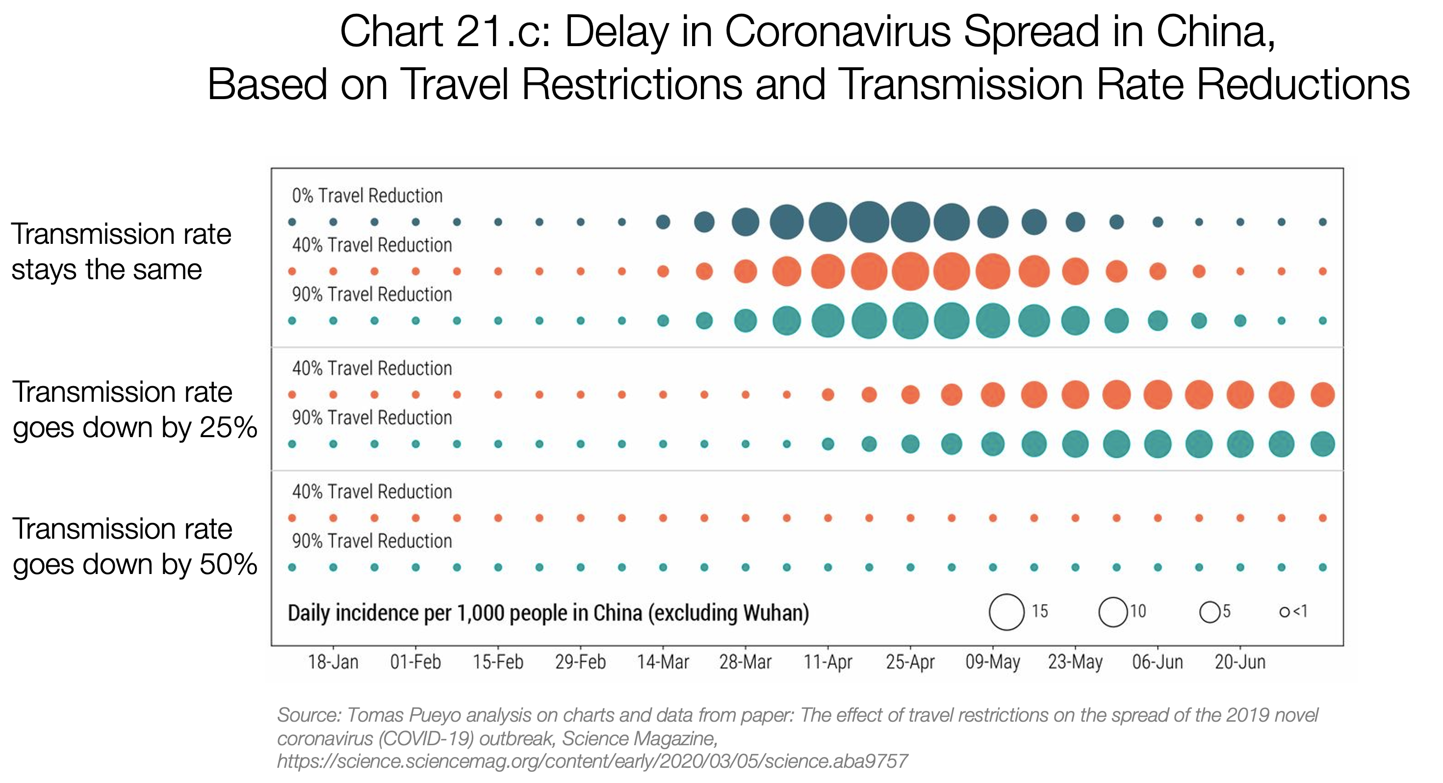
Together with what we have seen from the SIR modeling, reducing the transmission rate, and keeping the number of compartment small is crucial to flattening the curve. All should act together and fight the pandemic!
References
[1] https://www.vox.com/2020/2/18/21142009/coronavirus-covid19-china-wuhan-deaths-pandemic
[2] https://www.kaggle.com/allen-institute-for-ai/CORD-19-research-challenge
[3] https://github.com/CSSEGISandData/COVID-19/tree/master/csse_covid_19_data/csse_covid_19_time_series
[4] https://github.com/CSSEGISandData/COVID-19/tree/web-data
[5] http://gabgoh.github.io/COVID/index.html
[6] https://scipython.com/book/chapter-8-scipy/additional-examples/the-sir-epidemic-model/
[7] https://www.lewuathe.com/covid-19-dynamics-with-sir-model.html
[8] https://github.com/Lewuathe/COVID19-SIR
[9] https://en.wikipedia.org/wiki/2020_coronavirus_pandemic_in_India
[10] https://medium.com/@tomaspueyo/coronavirus-act-today-or-people-will-die-f4d3d9cd99ca
[11] https://science.sciencemag.org/content/early/2020/03/05/science.aba9757
[12] https://en.wikipedia.org/wiki/Compartmental_models_in_epidemiology
[13] https://science.sciencemag.org/content/early/2020/03/05/science.aba9757/tab-figures-data
[15] https://www.arcgis.com/apps/opsdashboard/index.html#/bda7594740fd40299423467b48e9ecf6
[16] https://www.weforum.org/agenda/2020/03/covid19-coronavirus-countries-infection-trajectory/