Introduction
Pipeline of activities in a typical machine learning project involves data preprocessing, exploratory data analysis, feature selection/feature engineering, model selection, hyper parameter tuning, generating model explanation and model selection/evaluation. This is an iterative process and data scientists spend a lot of time going through multiple iterations of this pipeline before they are able to identify the best model. AutoML aims to automates this workflow.
arcgis.learn users will now be able to use AutoML for supervised learning classification or regression problems involving tabular data. The AutoML implementation in arcgis.learn builds upon the implementation from MLJar (https://github.com/mljar/mljar-supervised)
Prepare tabular data
Data can be feature layer, spatially enabled dataframe with/without rasters or just a simple dataframe. The data for AutoML is prepared the same way it is prepared for supervised learning ML Models.
%matplotlib inline

from IPython.display import Image, HTML
import arcgis
from arcgis.gis import GIS
from arcgis.learn import prepare_tabulardata,AutoML
from sklearn.preprocessing import MinMaxScaler,RobustScaler
Here we will be taking a feature layer hosted on ArcGIS Online, convert it to a spatially enabled dataframe and prepare the data using prepare_tabulardata method from arcgis.learn. More details about data preparation for ML Models can be found here
gis = GIS('home')calgary_no_southland_solar = gis.content.search('calgary_no_southland_solar owner:api_data_owner', 'feature layer')[0]
calgary_no_southland_solar
calgary_no_southland_solar_layer = calgary_no_southland_solar.layers[0]
calgary_no_southland_solar_layer_sdf = calgary_no_southland_solar_layer.query().sdf
calgary_no_southland_solar_layer_sdf=calgary_no_southland_solar_layer_sdf[['FID','date','ID','solar_plan','altitude_m',
                                                                           'latitude','longitude','wind_speed','dayl__s_',
                                                                           'prcp__mm_d','srad__W_m_','swe__kg_m_', 'tmax__deg',
                                                                           'tmin__deg','vp__Pa_','kWh_filled','capacity_f',
                                                                           'SHAPE']]
calgary_no_southland_solar_layer_sdf.head()| FID | date | ID | solar_plan | altitude_m | latitude | longitude | wind_speed | dayl__s_ | prcp__mm_d | srad__W_m_ | swe__kg_m_ | tmax__deg | tmin__deg | vp__Pa_ | kWh_filled | capacity_f | SHAPE | |
|---|---|---|---|---|---|---|---|---|---|---|---|---|---|---|---|---|---|---|
| 0 | 1 | 2017-12-24 | 355827 | Glenmore Water Treatment Plant | 1095 | 51.003078 | -114.100571 | 7.20467 | 27648.0 | 1 | 108.800003 | 12 | -10.5 | -21.0 | 120 | 1.242357 | 0.000177 | {"x": -12701617.407282012, "y": 6621838.159138... |
| 1 | 2 | 2017-12-25 | 355827 | Glenmore Water Treatment Plant | 1095 | 51.003078 | -114.100571 | 3.385235 | 27648.0 | 1 | 115.199997 | 12 | -18.0 | -29.5 | 40 | 2.477714 | 0.000354 | {"x": -12701617.407282012, "y": 6621838.159138... |
| 2 | 3 | 2017-12-26 | 355827 | Glenmore Water Treatment Plant | 1095 | 51.003078 | -114.100571 | 5.076316 | 27648.0 | 0 | 118.400002 | 12 | -20.0 | -32.0 | 40 | 3.713071 | 0.00053 | {"x": -12701617.407282012, "y": 6621838.159138... |
| 3 | 4 | 2017-12-27 | 355827 | Glenmore Water Treatment Plant | 1095 | 51.003078 | -114.100571 | 5.617623 | 27648.0 | 0 | 96.0 | 12 | -18.0 | -26.5 | 80 | 4.948429 | 0.000707 | {"x": -12701617.407282012, "y": 6621838.159138... |
| 4 | 5 | 2017-12-28 | 355827 | Glenmore Water Treatment Plant | 1095 | 51.003078 | -114.100571 | 2.561512 | 27648.0 | 0 | 118.400002 | 12 | -17.0 | -28.5 | 40 | 6.183786 | 0.000883 | {"x": -12701617.407282012, "y": 6621838.159138... |
X = ['altitude_m', 'wind_speed', 'dayl__s_', 'prcp__mm_d','srad__W_m_','swe__kg_m_','tmax__deg','tmin__deg','vp__Pa_']
preprocessors =  [('altitude_m', 'wind_speed', 'dayl__s_', 'prcp__mm_d','srad__W_m_','swe__kg_m_','tmax__deg',
                   'tmin__deg','vp__Pa_', RobustScaler())]
data = prepare_tabulardata(calgary_no_southland_solar_layer,
'capacity_f',
explanatory_variables=X,
preprocessors=preprocessors)Train model using AutoML
from arcgis.learn import AutoMLAutoML class accepts the following paramters:
-
data (Required Paramter): Returned data object from
prepare_tabulardatafunction in the previous step. -
total_time_limit (Optional parameter): It is the total time in seconds that must be used for AutoML training. Default set is 3600 (1 Hr). At the completion of total_time_limit, the training of AutoML completes and the best model trained until then is used.
-
mode (Optional Parameter): Model can be either Explain. Perform or Compete. Default is Explain.
-
algorithms (Optional Parameter): This parameter takes in list of algorithms as input. The algorithms could be subset of the following: Linear,Decision Tree,Random Forest,Extra Trees,LightGBM,Xgboost,Neural Network.
-
eval_metric (Optional Parameter): The metric to be used to compare models.
AutoML modes
- Explain : To to be used when you want to explain and understand the data. Uses 75%/25% train/test split. Uses the following models: Baseline, Linear, Decision Tree, Random Forest, XGBoost, Neural Network, and Ensemble. Has full explanations in reports: learning curves, importance plots, and SHAP plots.
- Perform : To be used when you want to train a model that will be used in real-life use cases. Uses 5-fold CV (Cross-Validation). Uses the following models: Linear, Random Forest, LightGBM, XGBoost,Neural Network, and Ensemble. Has learning curves and importance plots in reports.
- Compete : To be used for machine learning competitions (maximum performance). Uses 10-fold CV (Cross-Validation). Uses the following models: Decision Tree, Random Forest, Extra Trees, XGBoost, Neural Network, Nearest Neighbors, Ensemble, and Stacking.It has only learning curves in the reports.
AutoML_class_obj = AutoML(data=data)After creating the AutoML object by passing the data obtained from prepare_tabulardata and using default values for other parameters, now we proceed to train the model using AutoML. This is done by calling the fit method as shown below. New folder will be created and all the models and their varients are saved in that folder.
AutoML_class_obj.fit()Neural Network algorithm was disabled because it doesn't support n_jobs parameter. AutoML directory: ~\AppData\Local\Temp\scratch\tmpmbhb97_l The task is regression with evaluation metric rmse AutoML will use algorithms: ['Linear', 'Decision Tree', 'Random Trees', 'Extra Trees', 'LightGBM', 'Xgboost'] AutoML will ensemble available models AutoML steps: ['simple_algorithms', 'default_algorithms', 'ensemble'] * Step simple_algorithms will try to check up to 2 models 1_DecisionTree rmse 0.048893 trained in 3.63 seconds Exception while producing SHAP explanations. 'float' object has no attribute 'shape' Continuing ... 2_Linear rmse 0.046288 trained in 1.1 seconds * Step default_algorithms will try to check up to 4 models 3_Default_LightGBM rmse 0.028985 trained in 7.23 seconds There was an error during 4_Default_Xgboost training. Please check ~\AppData\Local\Temp\scratch\tmpmbhb97_l\errors.md for details. 5_Default_RandomTrees rmse 0.043642 trained in 4.5 seconds 6_Default_ExtraTrees rmse 0.044894 trained in 6.55 seconds * Step ensemble will try to check up to 1 model Ensemble rmse 0.028985 trained in 0.28 seconds AutoML fit time: 32.35 seconds AutoML best model: 3_Default_LightGBM All the evaluated models are saved in the path ~\AppData\Local\Temp\scratch\tmpmbhb97_l
Once the best model is identified after the completion of fit method, the model is then saved by calling the save method. The transforms and the encoders used on the training data, along with the Esri Model Definition (EMD) file and the dlpk is then saved in the path specified by the user.
AutoML_class_obj.save('AutoML_class_obj')We can get the score of the best model, visualize the results on validation dataset and also get predictions on new data using the corresponding methods shown below.
AutoML_class_obj.score()0.962025310798984
AutoML_class_obj.show_results()| altitude_m | capacity_f | dayl__s_ | prcp__mm_d | srad__W_m_ | swe__kg_m_ | tmax__deg | tmin__deg | vp__Pa_ | wind_speed | capacity_f_results | |
|---|---|---|---|---|---|---|---|---|---|---|---|
| 1489 | 1055 | 0.019555 | 29376.0 | 0 | 96.0 | 0 | -4.5 | -12.0 | 240 | 5.819128 | 0.017498 |
| 3502 | 1112 | 0.253015 | 53568.0 | 0 | 473.600006 | 0 | 24.5 | 8.0 | 680 | 5.097813 | 0.019465 |
| 4304 | 1070 | 0.248061 | 50112.0 | 0 | 422.399994 | 0 | 29.0 | 7.5 | 800 | 3.733651 | 0.021266 |
| 5491 | 1090 | 0.018597 | 34905.601562 | 0 | 265.600006 | 28 | 3.0 | -14.5 | 200 | 8.435382 | 0.016190 |
| 7679 | 1096 | 0.112015 | 44582.398438 | 0 | 288.0 | 0 | 22.5 | 10.5 | 1280 | 4.886889 | 0.015759 |
AutoML_class_obj.predict(data._dataframe.iloc[:100][X],prediction_type="dataframe")| altitude_m | wind_speed | dayl__s_ | prcp__mm_d | srad__W_m_ | swe__kg_m_ | tmax__deg | tmin__deg | vp__Pa_ | prediction_results | |
|---|---|---|---|---|---|---|---|---|---|---|
| 0 | 1095 | 7.20467 | 27648.0 | 1 | 108.800003 | 12 | -10.5 | -21.0 | 120 | -0.002004 |
| 1 | 1095 | 3.385235 | 27648.0 | 1 | 115.199997 | 12 | -18.0 | -29.5 | 40 | 0.000117 |
| 2 | 1095 | 5.076316 | 27648.0 | 0 | 118.400002 | 12 | -20.0 | -32.0 | 40 | 0.001523 |
| 3 | 1095 | 5.617623 | 27648.0 | 0 | 96.0 | 12 | -18.0 | -26.5 | 80 | 0.000313 |
| 4 | 1095 | 2.561512 | 27648.0 | 0 | 118.400002 | 12 | -17.0 | -28.5 | 40 | 0.000577 |
| ... | ... | ... | ... | ... | ... | ... | ... | ... | ... | ... |
| 95 | 1095 | 3.887439 | 50457.601562 | 0 | 419.200012 | 0 | 26.0 | 8.0 | 1080 | 0.218459 |
| 96 | 1095 | 5.680981 | 50457.601562 | 0 | 435.200012 | 0 | 31.5 | 10.0 | 1240 | 0.229766 |
| 97 | 1095 | 5.332447 | 50112.0 | 3 | 195.199997 | 0 | 21.0 | 12.0 | 1400 | 0.131819 |
| 98 | 1095 | 5.281691 | 49766.398438 | 7 | 288.0 | 0 | 24.5 | 9.0 | 1160 | 0.130322 |
| 99 | 1095 | 5.033775 | 49766.398438 | 1 | 384.0 | 0 | 24.0 | 8.5 | 1120 | 0.182289 |
100 rows × 10 columns
As in the case of MLModel and FullyConnectedNetwork, predictions can also be obtained in the form of feature class and rasters.
Additionally it is also possible to generate and view the report of all the models trained by the AutoML, the performance and the hyperparamters used in each of the model variant. The report can be generated using the report method as shown below. The reports, also show the learning curves and feature importance charts for each of the model evaluated during the training.
AutoML_class_obj.report()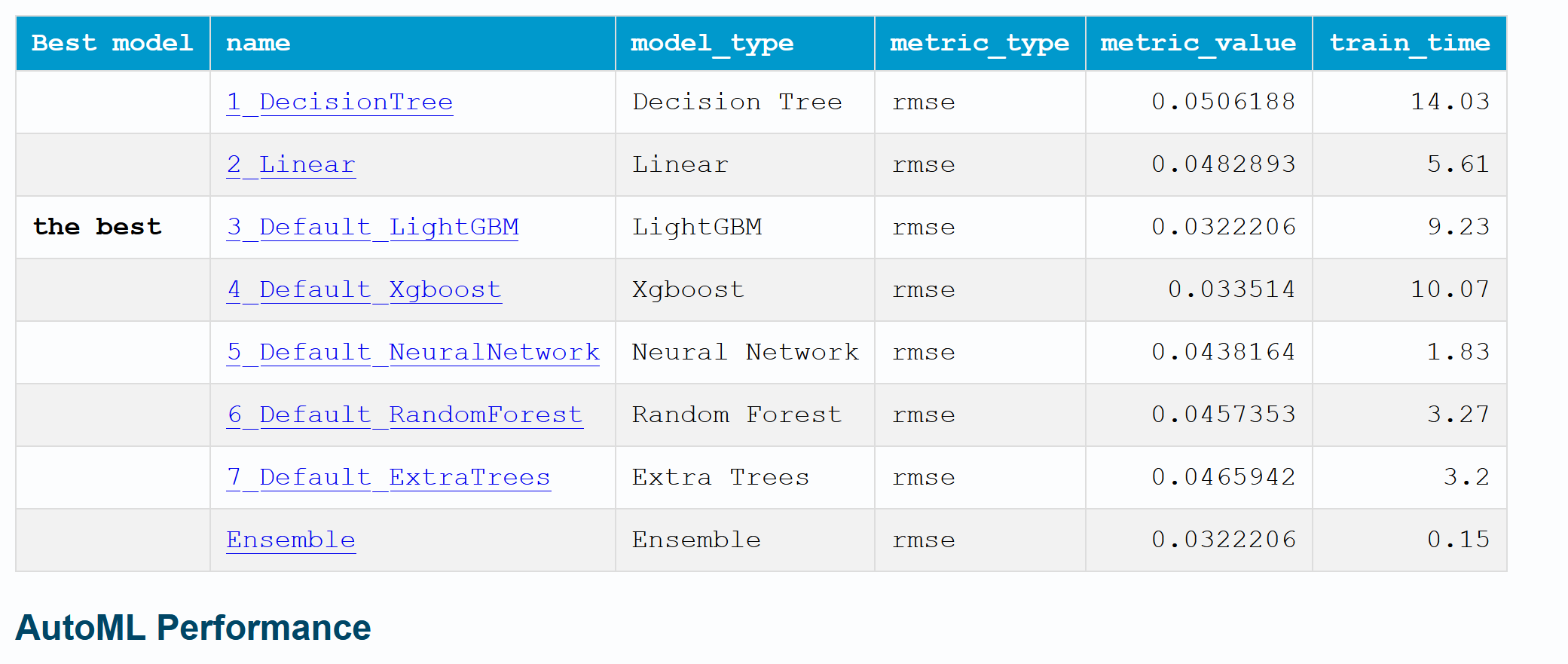
Reload trained model for prediction
The trained AutoML can be reloaded from the disk to get the predictions on new data. This is done using from_model method. This method takes in the path to the emd file as the input. The best model that was identified using the training phase will automatically be picked up and the prediction can be done on the new data using this model by calling the predict method.
from arcgis.learn import AutoML
AutoML_test_reload=AutoML.from_model(r'AutoML_class_obj')AutoML_test_reload.predict(data._dataframe.iloc[:100],prediction_type="dataframe")| altitude_m | capacity_f | dayl__s_ | prcp__mm_d | srad__W_m_ | swe__kg_m_ | tmax__deg | tmin__deg | vp__Pa_ | wind_speed | prediction_results | |
|---|---|---|---|---|---|---|---|---|---|---|---|
| 0 | 1095 | 0.000177 | 27648.0 | 1 | 108.800003 | 12 | -10.5 | -21.0 | 120 | 7.20467 | -0.002004 |
| 1 | 1095 | 0.000354 | 27648.0 | 1 | 115.199997 | 12 | -18.0 | -29.5 | 40 | 3.385235 | 0.000117 |
| 2 | 1095 | 0.00053 | 27648.0 | 0 | 118.400002 | 12 | -20.0 | -32.0 | 40 | 5.076316 | 0.001523 |
| 3 | 1095 | 0.000707 | 27648.0 | 0 | 96.0 | 12 | -18.0 | -26.5 | 80 | 5.617623 | 0.000313 |
| 4 | 1095 | 0.000883 | 27648.0 | 0 | 118.400002 | 12 | -17.0 | -28.5 | 40 | 2.561512 | 0.000577 |
| ... | ... | ... | ... | ... | ... | ... | ... | ... | ... | ... | ... |
| 95 | 1095 | 0.242472 | 50457.601562 | 0 | 419.200012 | 0 | 26.0 | 8.0 | 1080 | 3.887439 | 0.218459 |
| 96 | 1095 | 0.226795 | 50457.601562 | 0 | 435.200012 | 0 | 31.5 | 10.0 | 1240 | 5.680981 | 0.229766 |
| 97 | 1095 | 0.136033 | 50112.0 | 3 | 195.199997 | 0 | 21.0 | 12.0 | 1400 | 5.332447 | 0.131819 |
| 98 | 1095 | 0.139699 | 49766.398438 | 7 | 288.0 | 0 | 24.5 | 9.0 | 1160 | 5.281691 | 0.130322 |
| 99 | 1095 | 0.190066 | 49766.398438 | 1 | 384.0 | 0 | 24.0 | 8.5 | 1120 | 5.033775 | 0.182289 |
100 rows × 11 columns