- 🔬 Data Science
- 🥠 Deep Learning and Image Captioning
Introduction and objective
Image caption, a concise textual summary that describes the content of an image, has applications in numerous fields such as scene classification, virtual assistants, image indexing, social media, for visually impaired persons and more.
Deep learning has been achieving superhuman level performance in computer vision tasks ranging from object detection to natural language processing. ImageCaptioner, which is a combination of both image and text, is a deep learning model that generates image captions of remote sensing image data.
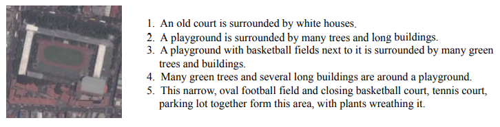
This sample shows how ArcGIS API for Python can be used to train ImageCaptioner model using Remote Sensing Image Captioning Dataset (RSICD) [1]. It is a publicly available dataset for remote sensing image captioning task. RSICD contains more than ten thousands remote sensing images which are collected from Google Earth, Baidu Map, MapABC and Tianditu. The images are fixed to 224X224 pixels with various resolutions. The total number of remote sensing images is 10921, with five sentences descriptions per image. The below screenshot shows an example of this data:
The trained model can be deployed on ArcGIS Pro or ArcGIS Enterprise to generate captions on a high satellite resolution imagery.
Necessary imports
from pathlib import Path
import os, json

from arcgis.learn import prepare_data, ImageCaptioner
from arcgis.gis import GIS
gis = GIS('home')Prepare data that will be used for training
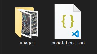
We need to put the RSICD dataset in a specific format, i.e., a root folder containing a folder named "images" and the JSON file containing the annotations named "annotations.json". The specific format of the json can be seen here.
Model training
Let's set a path to the folder that contains training images and their corresponding labels.
training_data = gis.content.get('8c4fc46930a044a9b20bb974d667e074')
training_data
filepath = training_data.download(file_name=training_data.name)import zipfile
with zipfile.ZipFile(filepath, 'r') as zip_ref:
zip_ref.extractall(Path(filepath).parent)data_path = Path(os.path.join(os.path.splitext(filepath)[0]))We'll use the prepare_data function to create a databunch with the necessary parameters such as batch_size, and chip_size. A complete list of parameters can be found in the API reference.
data = prepare_data(data_path,
                    chip_size=224,
                    batch_size=4,
                    dataset_type='ImageCaptioning')
Visualize training data
To visualize and get a sense of the training data, we can use the data.show_batch method.
data.show_batch()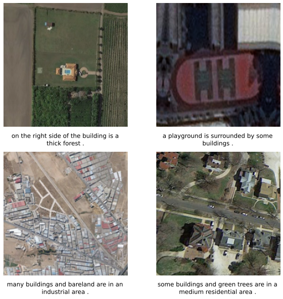
Load model architecture
arcgis.learn provides us image captioning model which are based on pretrained convnets, such as ResNet, that act as the backbones. We will use ImageCaptioner with the backbone parameters as Resnet50 to create our image captioning model. For more details on ImageCaptioner check out How image_captioning works? and the API reference.
ic = ImageCaptioner(data, backbone='resnet50')We will use the lr_find() method to find an optimum learning rate. It is important to set a learning rate at which we can train a model with good accuracy and speed.
lr = ic.lr_find()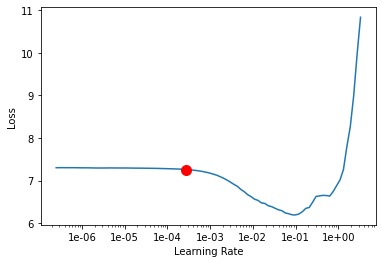
Train the model
We will now train the ImageCaptioner model using the suggested learning rate from the previous step. We can specify how many epochs we want to train for. Let's train the model for 100 epochs.
ic.fit(100, lr, early_stopping=True)| epoch | train_loss | valid_loss | accuracy | bleu | time |
|---|---|---|---|---|---|
| 0 | 4.695280 | 4.683484 | 0.169359 | 0.000000 | 53:17 |
| 1 | 4.149865 | 4.193302 | 0.212167 | 0.000000 | 53:33 |
| 2 | 3.847940 | 3.863936 | 0.302988 | 0.062242 | 53:08 |
| 3 | 3.531038 | 3.593763 | 0.350844 | 0.089471 | 53:07 |
| 4 | 3.237615 | 3.324673 | 0.380708 | 0.107219 | 53:04 |
| 5 | 2.885094 | 3.115619 | 0.413582 | 0.128764 | 53:05 |
| 6 | 2.745963 | 2.863758 | 0.445932 | 0.152206 | 53:10 |
| 7 | 2.540881 | 2.766686 | 0.462775 | 0.177337 | 53:09 |
| 8 | 2.355527 | 2.600504 | 0.489885 | 0.207568 | 53:06 |
| 9 | 2.313179 | 2.487214 | 0.504936 | 0.235590 | 53:04 |
| 10 | 2.054211 | 2.346865 | 0.529235 | 0.254470 | 53:10 |
| 11 | 2.047108 | 2.199641 | 0.551783 | 0.283868 | 53:10 |
| 12 | 2.064740 | 2.172241 | 0.556525 | 0.291952 | 53:06 |
| 13 | 1.986457 | 2.128242 | 0.563766 | 0.296588 | 53:06 |
| 14 | 1.826541 | 2.031750 | 0.579189 | 0.311093 | 53:11 |
| 15 | 1.763997 | 2.046451 | 0.566121 | 0.291099 | 53:05 |
| 16 | 1.817860 | 1.919416 | 0.592966 | 0.326027 | 53:06 |
| 17 | 1.766880 | 1.871730 | 0.592674 | 0.319502 | 53:58 |
| 18 | 1.714902 | 1.899555 | 0.593588 | 0.329748 | 53:33 |
| 19 | 1.617795 | 1.881732 | 0.595126 | 0.329128 | 53:17 |
| 20 | 1.604728 | 1.855326 | 0.600784 | 0.330772 | 53:13 |
| 21 | 1.565843 | 1.844262 | 0.603579 | 0.337001 | 53:16 |
| 22 | 1.554246 | 1.790282 | 0.609448 | 0.341711 | 53:15 |
| 23 | 1.581763 | 1.795434 | 0.613312 | 0.348124 | 53:32 |
| 24 | 1.543676 | 1.773622 | 0.615620 | 0.348699 | 53:47 |
| 25 | 1.504090 | 1.731651 | 0.625233 | 0.360189 | 53:47 |
| 26 | 1.532415 | 1.756249 | 0.615012 | 0.340073 | 53:10 |
| 27 | 1.473316 | 1.719556 | 0.620736 | 0.349469 | 53:05 |
| 28 | 1.420376 | 1.727326 | 0.616957 | 0.344545 | 53:05 |
| 29 | 1.487180 | 1.737915 | 0.622099 | 0.362117 | 53:05 |
| 30 | 1.449937 | 1.751929 | 0.618553 | 0.347141 | 53:08 |
| 31 | 1.485789 | 1.755898 | 0.624464 | 0.363179 | 53:08 |
| 32 | 1.371849 | 1.719512 | 0.621808 | 0.355478 | 53:08 |
Epoch 33: early stopping
Visualize results on validation set
To see sample results we can use the show_results method. This method displays the chips from the validation dataset with ground truth (left) and predictions (right). This visual analysis helps in assessing the qualitative results of the trained model.
ic.show_results()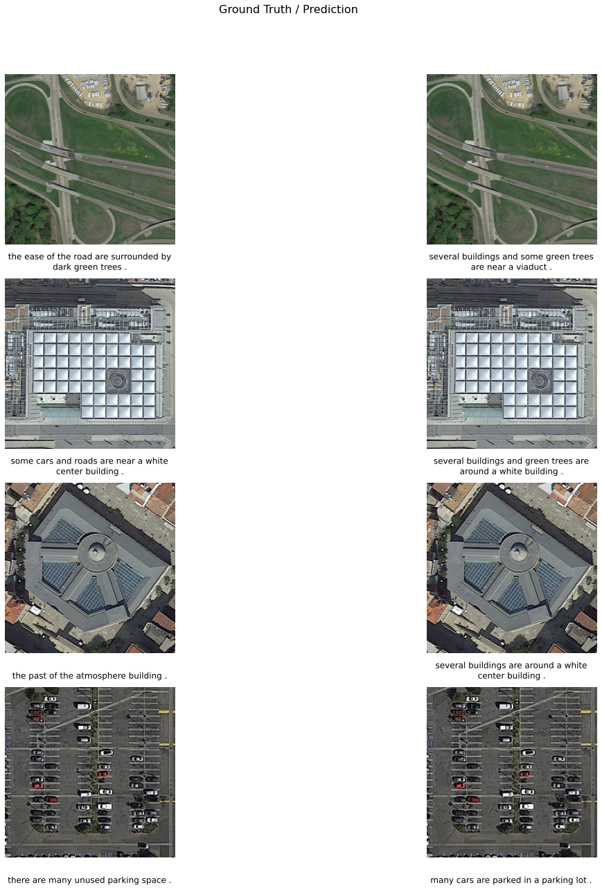
Evaluate model performance
To see the quantitative results of our model we will use the bleu_score method. Bilingual Evaluation Understudy Score(BLEU’s): is a popular metric that measures the number of sequential words that match between the predicted and the ground truth caption. It compares n-grams of various lengths from 1 through 4 to do this. A perfect match results in a score of 1.0, whereas a perfect mismatch results in a score of 0.0. summarizes how close the generated text is to the expected text.
ic.bleu_score(){'bleu-1': 0.5853038148042357,
'bleu-2': 0.3385487762905085,
'bleu-3': 0.2464713554187269,
'bleu-4': 0.1893991004368455,
'BLEU': 0.2583728068745172}Save the model
Let's save the model by giving it a name and calling the save method, so that we can load it later whenever required. The model is saved by default in a directory called models in the data_path initialized earlier, but a custom path can be provided.
ic.save('image-captioner-33epochs')Computing model metrics...
WindowsPath('//ImageCaptioning/models/image-captioner-33epochs')Prediction on test image
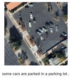
We can perform inferencing on a small test image using the predict function.
ic.predict(r'\image-captioner\test_img.tif')'some cars are parked in a parking lot .'
Now that we are satisfied with the model performance on a test image, we are ready to perform model inferencing on our desired images. In our case, we are interested in inferencing on high resolution satellite image.
Model inference
Before using the model for inference we need to make some changes in the model_name>.emd file. You can learn more about this file here.
By default, CropSizeFixed is set to 1. We want to change the CropSizeFixed to 0 so that the size of tile cropped around the features is not fixed. the below code will edit the emd file with CropSizeFixed:0 information.
with open(
    os.path.join(data_path, "models", "image-captioner-33epochs", "image-captioner-33epochs" + ".emd"), "r+"
) as emd_file:
    data = json.load(emd_file)
    data["CropSizeFixed"] = 0
    emd_file.seek(0)
    json.dump(data, emd_file, indent=4)
    emd_file.truncate()
In order to perform inferencing in ArcGIS Pro, we need to create a feature class on the map using Create Feature Class or Create Fishnet tool.
The Feature Class and the trained model has been provided for reference. You could directly download these files to run perform model inferencing on desired area.
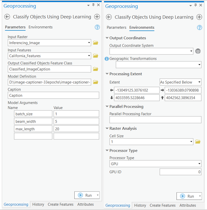
with arcpy.EnvManager(extent="-13049125.3076102 4033595.5228646 -13036389.0790898 4042562.3896354", cellSize=1, processorType="GPU"):
arcpy.ia.ClassifyObjectsUsingDeepLearning("Inferencing_Image", r"C:\Users\Admin\Documents\ImgCap\captioner.gdb\Classified_ImageCaptions", r"D:\image-captioner-33epochs\image-captioner-33epochs.emd", "California_Features", '', "PROCESS_AS_MOSAICKED_IMAGE", "batch_size 1;beam_width 5;max_length 20", "Caption")
Results
We selected an area unseen (by the model) and generated some features using the Create Feature Class tool. We then used our model to generate captions. Below are the results that we have achieved.
Conclusion
In this notebook, we demonstrated how to use the ImageCaptioner model from the ArcGIS API for Python to generate image captions using RSICD as training data.
References
- [1] Xiaoqiang Lu, Binqiang Wang, Xiangtao Zheng, Xuelong Li: “Exploring Models and Data for Remote Sensing Image Caption Generation”, 2017; arXiv:1712.07835. DOI: 10.1109/TGRS.2017.2776321.
- https://developers.arcgis.com/python/guide/how-image-captioning-works/