Introduction
We live in the digital era of smart devices, Internet of things (IoT), and Mobile solutions, where data has become an essential aspect of any enterprise. It is now crucial to gather, process, and analyze large volumes of data as quickly and accurately as possible.
Python has become one of the most popular programming languages for data science, machine learning, and general software development in academia and industry. It boasts a relatively low learning curve, due to its simplicity, and a large ecosystem of data-oriented libraries that can speed up and simplify numerous tasks.
When you are getting started, the vastness of Python may seem overwhelming, but it is not as complex as it seems. Python has also developed a large and active data analysis and scientific computing community, making it one of the most popular choices for data science. Using Python within ArcGIS enables you to easily work with open-source python libraries as well as with ArcGIS Python libraries.
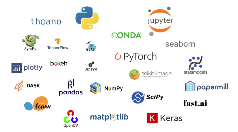
The image above shows some of the popular libraries in the Python ecosystem. This is by no means a full list, as the Python ecosystem is continuously evolving with numerous other libraries. Let's look at some of the popular libraries in the scientific Python ecosystem.
Libraries in Scientific Python Ecosystem
Data engineering is one of the most critical and foundational skills in any data scientist’s toolkit. A data scientist needs to get the data, clean and process it, visualize the results, and then model the data to analyze and interpret trends or patterns for making critical business decisions. The availability of various multi-purpose, ready-to-use libraries to perform these tasks makes Python a top choice for analysts, researchers, and scientists alike.
Data Processing
Data Processing is a process of cleaning and transforming data. It enables users to explore and discover useful information for decision-making. Some of the key Python libraries used for Data Processing are:
-
NumPy, short for Numerical Python, has been designed specifically for mathematical operations. It is a perfect tool for scientific computing and performing basic and advanced array operations. It primarily supports multi-dimensional arrays and vectors for complex arithmetic operations. In addition to the data structures, the library has a rich set of functions to perform algebraic operations on the supported data types. NumPy arrays form the core of nearly the entire ecosystem of data science tools in Python and are more efficient for storing and manipulating data than the other built-in Python data structures. NumPy’s high level syntax makes it accessible and productive for programmers from any background or experience level.
-
SciPy the Scientific Python library is a collection of numerical algorithms and domain-specific toolboxes. SciPy extends capabilities of NumPy by offering advanced modules for linear algebra, integration, optimization, and statistics. Together NumPy and SciPy form a reasonably complete and mature computational foundation for many scientific computing applications.
-
Pandas provides high-level data structures and functions designed to make working with structured or tabular data fast, easy, and expressive. Pandas blends the high-performance, array-computing ideas of NumPy with the flexible data manipulation capabilities of relational databases (such as SQL). It is based on two main data structures: "Series" (one-dimensional such as a list of items) and "DataFrames" (two-dimensional, such as a table). Pandas provides sophisticated indexing functionality to reshape, slice and dice, perform aggregations, and select subsets of data. It provides capabilities for easily handling missing data, adding/deleting columns, imputing missing data, and creating plots on the go. Pandas is a must-have tool for data wrangling and manipulation.
Data Visualization
An essential function of data analysis and exploration is to visualize data. Visualization makes it easier for the human brain to detect patterns, trends, and outliers in the data. Some of the key Python libraries used for Data Visualization are:
-
Matplotlib is the most popular Python library for producing plots and other two-dimensional data visualizations. It can be used to generate various types of graphs such as histograms, pie-charts, or a simple bar chart. Matplotlib is highly flexible, offering the ability to customize almost every available feature. It provides an object oriented, MATLAB-like interface for users, and as such, has generally good integration with the rest of the ecosystem.
-
Seaborn is based on Matplotlib and serves as a useful tool for making attractive and informative statistical graphics in Python. It can be used for visualizing statistical models, summarizing data, and depicting the overall distributions. Seaborn works with the dataset as a whole and is much more intuitive than Matplotlib. It automates the creation of various plot types and creates beautiful graphics. Simply importing seaborn improves the visual aesthetics of Matplotlib plots.
-
Bokeh is a great tool for creating interactive and scalable visualizations inside browsers using JavaScript widgets. It is an advanced library that is fully independent of Matplotlib. Bokeh's emphasis on widgets allows users to represent the data in various formats such as graphs, plots, and labels. It empowers the user to generate elegant and concise graphics in the style of D3.js. Bokeh has the capability of high-performance interactivity over very large datasets.
Data Modeling
The process of modeling involves training a machine learning algorithm. The output from modeling is a trained model that can be used for inference and for making predictions. Some of the key Python libraries used for Data Modeling are:
-
Scikit-Learn has become the industry standard and is a premier general-purpose machine learning toolkit for Python programmers. Built on NumPy, SciPy and matplotlib, it features algorithms for various machine learning, statistical modeling and data mining tasks. Scikit-Learn contains submodules for tasks such as preprocessing, classification, regression, model selection, dimensionality reduction as well as clustering. The library comes with sample datasets for users to experiment.
-
StatsModels is a statistical analysis package that contains algorithms for classical statistics and econometrics. It provides a complement to scipy for statistical computations and is more focused on providing statistical inference, uncertainty estimates and p-values for parameters. StatsModels features submodules for various tasks such as Regression Analysis, Analysis of Variance (ANOVA), Time Series Analysis, Non-parametric methods and Visualization of model results.
In this guide series, we will focus on two key libraries in the scientific Python ecosystem that are used for data processing, NumPy and Pandas. Before we go into the details of these two topics, we will briefly discuss Spatially Enabled DataFrame.
Spatially Enabled DataFrame
What is a DataFrame?
A DataFrame represents a rectangular table of data and contains an ordered collection of columns. You can think of it as a spreadsheet or SQL table where each column has a column name for reference, and each row can be accessed by using row numbers. Column names and row numbers are known as column and row indexes.
DataFrame is a fundamental Pandas data structure in which each column can be of a different value type (numeric, string, boolean, etc.). A data set can be first read into a DataFrame, and then various operations (i.e. indexing, grouping, aggregation etc.) can be easily applied to it.
Given some data, let's look at how a dataset can be read into a DataFrame to see what a DataFrame looks like.
# Data Creation
data = {'state':['CA','WA','CA','WA','CA','WA'],
        'year':[2015,2015,2016,2016,2017,2017],
        'population':[3.5,2.5,4.5,3.0,5.0,3.25]}
# Read data into a dataframe
import pandas as pd
df = pd.DataFrame(data)
df| state | year | population | |
|---|---|---|---|
| 0 | CA | 2015 | 3.50 |
| 1 | WA | 2015 | 2.50 |
| 2 | CA | 2016 | 4.50 |
| 3 | WA | 2016 | 3.00 |
| 4 | CA | 2017 | 5.00 |
| 5 | WA | 2017 | 3.25 |
You can see the tabular structure of data with indexed rows and columns. We will dive deeper into DataFrame in the
Introduction to Pandaspart of the guide series.
What is a Spatially Enabled DataFrame (SEDF)?
The Spatially Enabled DataFrame (SEDF) inserts "spatial abilities" into the popular Pandas DataFrame. This allows users to use intuitive Pandas operations on both the attribute and spatial columns. With SEDF, you can easily manipulate geometric and attribute data. SEDF is a capability that is added to the Pandas DataFrame structure, by the ArcGIS API for Python, to give it spatial abilities.
SEDF is based on data structures inherently suited to data analysis, with natural operations for the filtering and inspecting of subsets of values, which are fundamental to statistical and geographic manipulations.
Let's quickly look at how data can be imported and exported using Spatially Enabled DataFrame. The details shown below are a high level overview and we will take a deeper dive into working with Spatially Enabled DataFrame in the later parts of this guide series.
Reading Data into Spatially Enabled DataFrame
Spatially Enabled DataFrame (SEDF) can read data from many sources, including:
SEDF integrates with Esri's ArcPy site-package as well as with the open source pyshp, shapely and fiona packages. This means that SEDF can use either of these geometry engines to provide you options for easily working with geospatial data regardless of your platform.
Exporting Data from Spatially Enabled DataFrame
The SEDF can export data to various data formats for use in other applications. Export options are:
Quick Example
Let's look at an example of utilizing Spatially Enabled DataFrame (SEDF) through the machine learning lifecycle. We will focus on the usage of SEDF through the process and not so much on the intepretation or results of the model. The example shows how to:
- Read data from Pandas DataFrame into a SEDF.
- Use SEDF with other libraries in python ecosystem for modeling and predictions.
- Merge modeled results back into SEDF.
- Export data from a SEDF.
We will use a subset of Covid-19 Nursing Home data from Centers for Medicare & Medicaid Services (CMS) to illustrate this example. Note that the dataset used in this example has been curated for illustration purposes and does not reflect the complete dataset available at CMS website.
Goal: Predict "Total Number of Occupied Beds" using other variables in the data.
In this example, we will:
- Read the data (with location attributes) into a SEDF and plot SEDF on a map.
- Split SEDF into train and test sets.
- Build a linear regression model on training data.
- Get Predictions for the model using test data.
- Add Predictions back to SEDF.
- Plot SEDF with predicted data on a map.
- Export SEDF.
Read the Data
# Import Libraries
from IPython.display import display

import pandas as pd
from arcgis.gis import GIS
import geopandas
# Create a GIS Connection
gis = GIS(profile='your_online_profile')# Read the data
df = pd.read_csv('../data/sample_cms_data.csv')
# Return the first 5 records
df.head()| Provider Name | Provider City | Provider State | Residents Weekly Admissions COVID-19 | Residents Total Admissions COVID-19 | Residents Weekly Confirmed COVID-19 | Residents Total Confirmed COVID-19 | Residents Weekly Suspected COVID-19 | Residents Total Suspected COVID-19 | Residents Weekly All Deaths | Residents Total All Deaths | Residents Weekly COVID-19 Deaths | Residents Total COVID-19 Deaths | Number of All Beds | Total Number of Occupied Beds | LONGITUDE | LATITUDE | |
|---|---|---|---|---|---|---|---|---|---|---|---|---|---|---|---|---|---|
| 0 | GROSSE POINTE MANOR | NILES | IL | 3 | 5 | 10 | 56 | 0 | 10 | 6 | 15 | 4 | 12 | 99 | 61 | -87.792973 | 42.012012 |
| 1 | MILLER'S MERRY MANOR | DUNKIRK | IN | 0 | 0 | 0 | 0 | 0 | 0 | 0 | 0 | 0 | 0 | 46 | 43 | -85.197651 | 40.392722 |
| 2 | PARKWAY MANOR | MARION | IL | 0 | 0 | 0 | 0 | 0 | 0 | 0 | 0 | 0 | 0 | 131 | 84 | -88.982944 | 37.750143 |
| 3 | AVANTARA LONG GROVE | LONG GROVE | IL | 1 | 6 | 0 | 141 | 3 | 3 | 0 | 0 | 0 | 0 | 195 | 131 | -87.986442 | 42.160843 |
| 4 | HARMONY NURSING & REHAB CENTER | CHICAGO | IL | 2 | 19 | 1 | 75 | 0 | 0 | 0 | 43 | 0 | 16 | 180 | 116 | -87.726353 | 41.975505 |
# Get concise summary of the dataframe
df.info()
<class 'pandas.core.frame.DataFrame'> RangeIndex: 124 entries, 0 to 123 Data columns (total 17 columns): # Column Non-Null Count Dtype --- ------ -------------- ----- 0 Provider Name 124 non-null object 1 Provider City 124 non-null object 2 Provider State 124 non-null object 3 Residents Weekly Admissions COVID-19 124 non-null int64 4 Residents Total Admissions COVID-19 124 non-null int64 5 Residents Weekly Confirmed COVID-19 124 non-null int64 6 Residents Total Confirmed COVID-19 124 non-null int64 7 Residents Weekly Suspected COVID-19 124 non-null int64 8 Residents Total Suspected COVID-19 124 non-null int64 9 Residents Weekly All Deaths 124 non-null int64 10 Residents Total All Deaths 124 non-null int64 11 Residents Weekly COVID-19 Deaths 124 non-null int64 12 Residents Total COVID-19 Deaths 124 non-null int64 13 Number of All Beds 124 non-null int64 14 Total Number of Occupied Beds 124 non-null int64 15 LONGITUDE 124 non-null float64 16 LATITUDE 124 non-null float64 dtypes: float64(2), int64(12), object(3) memory usage: 16.6+ KB
The dataset contains 124 records and 17 columns. Each record represents a nursing home in the states of Indiana and Illinois. Each column contains information about the nursing home such as:
- Name of the nursing home, its city and its state
- Details of resident Covid cases, deaths and number of beds
- Location of nursing home as Latitude and Longitude
Read into Spatially Enabled Dataframe
Any Pandas DataFrame with location information (Latitude and Longitude) can be read into a Spatially Enabled DataFrame using the from_xy() method.
sedf = pd.DataFrame.spatial.from_xy(df,'LONGITUDE','LATITUDE')
sedf.head()| Provider Name | Provider City | Provider State | Residents Weekly Admissions COVID-19 | Residents Total Admissions COVID-19 | Residents Weekly Confirmed COVID-19 | Residents Total Confirmed COVID-19 | Residents Weekly Suspected COVID-19 | Residents Total Suspected COVID-19 | Residents Weekly All Deaths | Residents Total All Deaths | Residents Weekly COVID-19 Deaths | Residents Total COVID-19 Deaths | Number of All Beds | Total Number of Occupied Beds | LONGITUDE | LATITUDE | SHAPE | |
|---|---|---|---|---|---|---|---|---|---|---|---|---|---|---|---|---|---|---|
| 0 | GROSSE POINTE MANOR | NILES | IL | 3 | 5 | 10 | 56 | 0 | 10 | 6 | 15 | 4 | 12 | 99 | 61 | -87.792973 | 42.012012 | {"spatialReference": {"wkid": 4326}, "x": -87.... |
| 1 | MILLER'S MERRY MANOR | DUNKIRK | IN | 0 | 0 | 0 | 0 | 0 | 0 | 0 | 0 | 0 | 0 | 46 | 43 | -85.197651 | 40.392722 | {"spatialReference": {"wkid": 4326}, "x": -85.... |
| 2 | PARKWAY MANOR | MARION | IL | 0 | 0 | 0 | 0 | 0 | 0 | 0 | 0 | 0 | 0 | 131 | 84 | -88.982944 | 37.750143 | {"spatialReference": {"wkid": 4326}, "x": -88.... |
| 3 | AVANTARA LONG GROVE | LONG GROVE | IL | 1 | 6 | 0 | 141 | 3 | 3 | 0 | 0 | 0 | 0 | 195 | 131 | -87.986442 | 42.160843 | {"spatialReference": {"wkid": 4326}, "x": -87.... |
| 4 | HARMONY NURSING & REHAB CENTER | CHICAGO | IL | 2 | 19 | 1 | 75 | 0 | 0 | 0 | 43 | 0 | 16 | 180 | 116 | -87.726353 | 41.975505 | {"spatialReference": {"wkid": 4326}, "x": -87.... |
Spatially Enabled DataFrame (SEDF) adds spatial abilities to the data. A SHAPE column gets added to the dataset as it is read into a SEDF. We can now plot this DataFrame on a map.
Plot on a Map
m1 = gis.map('IL, USA')
m1
Points displayed on the map show the location of each nursing home in our data. Clicking on a point displays attribute information for that nursing home.
sedf.spatial.plot(m1)True
Split the Data
We will split the Spatially Enabled DataFrame into training and test datasets and separate out the predictor and response variables in training and test data.
# Split data into Train and Test Sets
from sklearn.model_selection import train_test_split
train_data, test_data = train_test_split(sedf, test_size=0.2, random_state=101)
# Look at shape of training and test datasets
print(f'Shape of training data: {train_data.shape}')
print(f'Shape of testing data: {test_data.shape}')Shape of training data: (99, 18) Shape of testing data: (25, 18)
Response Variable
Any regression prediction task requires a variable of interest, a variable we would like to predict. This variable is called as a Response variable, also referred to as y variable or Dependent variable. Our goal is to predict "Total Number of Occupied Beds", so our y variable will be "Total Number of Occupied Beds".
Predictor Variables
All other variables the affect the Response variable are called Predictor variables. These predictor variables are also known as x variables or Independent variables. In this example, we will use only numerical variables related to Covid cases, deaths and number of beds as x variables, and we will ignore provder details such as name, city, state or location information.
Here, we use Indexing to select specific columns from the DataFrame. We will talk about Indexing in more detail in the later sections of this guide series.
# Separate predictors and response variables for train and test data
train_x = train_data.iloc[:,3:-4]
train_y = train_data.iloc[:,-4]
test_x = test_data.iloc[:,3:-4]
test_y = test_data.iloc[:,-4]
Build the Model
We will build and fit a Linear Regression model using the LinearRegression() method from the Scikit-learn library. Our goal is to predict the total number of occupied beds.
# Build the model
from sklearn import linear_model

# Create linear regression object
lr_model = linear_model.LinearRegression()
# Train the model using the training sets
lr_model.fit(train_x, train_y)LinearRegression()
Get Predictions
We will now use the model to make predictions on our test data.
# Get predictions
bed_predictions = lr_model.predict(test_x)
bed_predictions
array([ 70.18799777, 79.35734213, 40.52267526, 112.32693137,
74.56730982, 92.59096106, 70.69189401, 29.84238321,
108.09537913, 81.10718742, 59.90388811, 67.44325594,
70.62977058, 96.44880679, 85.19537597, 39.10578923,
63.88519971, 76.36549693, 38.94543793, 41.96507956,
50.41997091, 66.00665849, 33.30750881, 75.17989671,
63.09585712])Add Predictions to Test Data
Here, we add predictions back to the test data as a new column, Predicted_Occupied_Beds. Since the test dataset is a Spatially Enabled DataFrame, it continues to provide spatial abilities to our data.
# Convert predictions into a dataframe
pred_available_beds = pd.DataFrame(bed_predictions, index = test_data.index,
                                   columns=['Predicted_Occupied_Beds'])
pred_available_beds.head()| Predicted_Occupied_Beds | |
|---|---|
| 74 | 70.187998 |
| 123 | 79.357342 |
| 78 | 40.522675 |
| 41 | 112.326931 |
| 79 | 74.567310 |
# Add predictions back to test dataset
test_data = pd.concat([test_data, pred_available_beds], axis=1)
test_data.head()| Provider Name | Provider City | Provider State | Residents Weekly Admissions COVID-19 | Residents Total Admissions COVID-19 | Residents Weekly Confirmed COVID-19 | Residents Total Confirmed COVID-19 | Residents Weekly Suspected COVID-19 | Residents Total Suspected COVID-19 | Residents Weekly All Deaths | Residents Total All Deaths | Residents Weekly COVID-19 Deaths | Residents Total COVID-19 Deaths | Number of All Beds | Total Number of Occupied Beds | LONGITUDE | LATITUDE | SHAPE | Predicted_Occupied_Beds | |
|---|---|---|---|---|---|---|---|---|---|---|---|---|---|---|---|---|---|---|---|
| 74 | GOLDEN YEARS HOMESTEAD | FORT WAYNE | IN | 0 | 5 | 0 | 0 | 0 | 0 | 0 | 0 | 0 | 0 | 110 | 104 | -85.036651 | 41.107479 | {"spatialReference": {"wkid": 4326}, "x": -85.... | 70.187998 |
| 123 | WATERS OF DILLSBORO-ROSS MANOR, THE | DILLSBORO | IN | 0 | 4 | 0 | 0 | 0 | 0 | 0 | 7 | 0 | 0 | 123 | 75 | -85.056649 | 39.018794 | {"spatialReference": {"wkid": 4326}, "x": -85.... | 79.357342 |
| 78 | TOWNE HOUSE RETIREMENT COMMUNITY | FORT WAYNE | IN | 0 | 0 | 1 | 1 | 1 | 1 | 0 | 1 | 0 | 0 | 58 | 46 | -85.111952 | 41.133477 | {"spatialReference": {"wkid": 4326}, "x": -85.... | 40.522675 |
| 41 | UNIVERSITY HEIGHTS HEALTH AND LIVING COMMUNITY | INDIANAPOLIS | IN | 0 | 0 | 0 | 0 | 0 | 0 | 0 | 8 | 0 | 0 | 174 | 133 | -86.135442 | 39.635530 | {"spatialReference": {"wkid": 4326}, "x": -86.... | 112.326931 |
| 79 | SHARON HEALTH CARE PINES | PEORIA | IL | 0 | 0 | 0 | 0 | 0 | 0 | 0 | 1 | 0 | 0 | 116 | 96 | -89.643629 | 40.731764 | {"spatialReference": {"wkid": 4326}, "x": -89.... | 74.567310 |
Plot on a Map
Here, we plot test_data on a map. The map shows the location of each nursing home in the test dataset, along with the attribute information. We can see model prediction results added as Predicted_Occupied_Beds column, along with the actual number of occupied beds, Total_Number_of_Occupied_Beds , in the test data.
m2 = gis.map('IL, USA')
m2
test_data.spatial.plot(m2)True
Export Data
We will now export the Spatially Enabled DataFrame test_data to a feature layer. The to_featurelayer() method allows us to publish spatially enabled DataFrame as feature layers to the portal.
lyr = test_data.spatial.to_featurelayer('sedf_predictions')
lyr
Conclusion
There are numerous libraries in the scientific python ecosystem. In this part of the guide series, we briefly discussed some of the key libraries used for data processing, visualization, and modeling. We introduced the concept of the Spatially Enabled DataFrame (SEDF) and how it adds "spatial" abilities to the data. You have also seen an end-to-end example of using SEDF through the machine learning lifecycle, starting from reading data into SEDF, to exporting a SEDF.
In the next part of this guide series, you will learn more about NumPy in the Introduction to NumPy section..
References
[1] Wes McKinney. 2017. Python for Data Analysis: Data Wrangling with Pandas, NumPy, and IPython (2nd. ed.). O'Reilly Media, Inc.
[2] Jake VanderPlas. 2016. Python Data Science Handbook: Essential Tools for Working with Data (1st. ed.). O'Reilly Media, Inc.