Introduction to NumPy
NumPy, short for Numerical Python, is the core library for scientific computing in Python. It has been designed specifically for performing basic and advanced array operations. It primarily supports multi-dimensional arrays and vectors for complex arithmetic operations. Here are some things you will find in NumPy:
-
ndarray, an efficient multidimensional array object providing fast array-oriented arithmetic operations and flexible broadcasting capabilities. -
Mathematical functions for fast operations on entire arrays of data without having to write loops.
-
Tools for reading/writing array data to disk and working with memory-mapped files.
-
Linear algebra, random number generation, and Fourier transform capabilities.
NumPy arrays form the core of nearly the entire ecosystem of data science tools in Python. They provide:
- Efficient storage and data operations as they use much less memory than built-in Python sequences.
- Ability to perform complex computations on large blocks of data without the need for using Python for loops.
- Performance as arrays are much faster than Python core library provided Lists.
NumPy by itself does not provide modeling or scientific functionality, but an understanding of NumPy arrays and array-oriented computing will help you use tools, such as pandas, much more effectively.
Installation and Import
A typical installation of Python API comes with Numpy. You can use pip or conda to install it.
# conda install numpy
# pip install numpy
Once NumPy is installed, you can import it as:
import numpy as npYou can also check the version of NumPy that is installed:
np.__version__'1.18.5'
Creating Arrays
One of the key features of NumPy is its N-dimensional array object ndarray. An ndarray is a generic multidimensional container for homogeneous data; that is, all of the elements in the array must be the same type. So, an array is like a grid of values, all of the same type. The values in an array are indexed by a tuple of nonnegative integers.
Creating N-dimensional Array
The easiest way to create an array is to use the array function. We can initialize numpy arrays from Python lists. Let's create one, two, and three dimensional arrays using lists.
# Create one-dimensional array
data1 = [1,2,3,6,7]
arr1 = np.array(data1)
arr1
array([1, 2, 3, 6, 7])
# Create two and three dimensional arrays
data2 = [[1,2,3,6], [2,6,9,11]]
data3 = [[[1, 2], [3, 4]], [[5, 6], [7, 8]]]

arr2 = np.array(data2)
arr3 = np.array(data3)

print('2D array:\n', arr2)
print('\n')
print('3D array:\n', arr3)
2D array: [[ 1 2 3 6] [ 2 6 9 11]] 3D array: [[[1 2] [3 4]] [[5 6] [7 8]]]
Creating arrays using random number generator
We can also generate arrays using NumPy's random number generator. Numpy's np.random module contains rand, randn and randint functions that can be used to generate different random numbers from different distributions.
rand- generates random samples from uniform distribution between 0 and 1. We specify the shape of the resulting array we want.randn- generates random samples from normal distribution with mean 0 and standard deviation 1. We specify the shape of the resulting array we want.randint- generates random integers from a given low and high value range. We specify the min and max values for random number generation and also the shape of the resulting array we want.
Let's create a 2-D array using rand.
# Arrays using rand
r1 = np.random.rand(2,4)
r1
array([[0.80668187, 0.04487517, 0.05382909, 0.79854817],
[0.64946385, 0.8975755 , 0.79676167, 0.53641035]])Now, let's create a 3-D array using randn.
# Arrays using rand
r2 = np.random.randn(2,3,2)
r2
array([[[ 0.76102009, -1.40584035],
[-1.29607784, 0.27082671],
[-0.32464382, -0.46424713]],
[[-2.13802959, 1.05216567],
[-0.37643712, 0.45702234],
[-0.74756525, 0.1225769 ]]])Let's create a 2-D array of random integers between 2 and 10 using randint.
r3 = np.random.randint(2,10, size=(2, 4))  # Two-dimensional array
r3
array([[2, 9, 7, 6],
[6, 3, 3, 6]])Attibutes of a NumPy Array
Each array has attributes such as:
ndim(the number of dimensions)shape(the size of each dimension)size(the total size of the array)dtype(the data type of the array)
Let's look at each of these attributes. We will use array r2 defined above to check these attributes. These attributes are extremely useful and come in handy during the data exploration phase of a project.
ndim: Number of dimensions
r2.ndim3
shape: Size of each dimension
r2.shape(2, 3, 2)
size: Total number of elements in the array
r2.size12
dtype: Data type of the array
r2.dtypedtype('float64')Navigating Arrays
Elements of an array can be accessed in multiple ways. We can use [] to access individual elements on an array. We can also use slice notation, marked by the colon (:) character to access subarrays. Indexing and slicing of NumPy arrays is very similar to Python Lists.
Array Indexing - Accessing Single Elements
In a one-dimensional array, the value can be accessed by specifying the desired index. In a multi-dimensional array, value can be accessed using a comma-separated indices. We will use arrays defined above to look at some examples.
# Print arrays
print('1D array:\n', arr1)
print('2D array:\n', arr2)
print('3D array:\n', arr3)
1D array: [1 2 3 6 7] 2D array: [[ 1 2 3 6] [ 2 6 9 11]] 3D array: [[[1 2] [3 4]] [[5 6] [7 8]]]
One-dimensional Array
# Access value at index 0
arr1[0]
1
# Access value at index 2
arr1[2]
3
To index from the end of the array, you can use negative indices.
arr1[-1]7
arr1[-3]3
Multi-dimensional Array
In a multi-dimensional array, the elements at each index are no longer scalars but rather sub-arrays. Elements of a multi-dimensional array can be accessed using a comma-separated list of indices. If you omit later indices, the returned object will be a sub-array. Let's take a look.
2-D Array
# Print array
arr2
array([[ 1, 2, 3, 6],
[ 2, 6, 9, 11]])# Access value at index [0]
arr2[0]array([1, 2, 3, 6])
Accessing
# Access value at index [0,0]
arr2[0,0]
1
# Access value at index [1,2]
arr2[1,2]
9
3-D Array
# Print array
arr3
array([[[1, 2],
[3, 4]],
[[5, 6],
[7, 8]]])# Access value at index [0]
arr3[0]array([[1, 2],
[3, 4]])Accessing
# Access a specific element
arr3[0,1,1]
4
Array Slicing
We can use slice notation, marked by the colon (:) character to access sub-arrays of ndarrays. To access a slice of an array x, we can use the NumPy slicing syntax x[start:stop:slice]. Let's look at accessing sub-arrays in one dimension and in multiple dimensions.
# Print arrays
print('1D array:\n', arr1)
print('2D array:\n', arr2)
print('3D array:\n', arr3)
1D array: [1 2 3 6 7] 2D array: [[ 1 2 3 6] [ 2 6 9 11]] 3D array: [[[1 2] [3 4]] [[5 6] [7 8]]]
One-dimensional Array
# first three elements
arr1[:3]
array([1, 2, 3])
# elements after index 2
arr1[2:]
array([3, 6, 7])
# middle sub-array
arr1[1:4]
array([2, 3, 6])
# every other element
arr1[::2]
array([1, 3, 7])
# all elements reversed
arr1[::-1]
array([7, 6, 3, 2, 1])
Multi-dimensional Array
Slices in a multi-dimensional array can be accessed using a comma-separated list of indices. If you omit later indices, the returned object will be a sub-array. Let's take a look.
# Print data
arr2
array([[ 1, 2, 3, 6],
[ 2, 6, 9, 11]])# two rows, two columns
arr2[:2, :2]array([[1, 2],
[2, 6]])# all rows, every other column
arr2[:, ::2]array([[1, 3],
[2, 9]])Indexing and Slicing can be combined to access single rows or columns on an array.
# first row
arr2[0, :]
array([1, 2, 3, 6])
# first column
arr2[:, 0]
array([1, 2])
Reshaping Arrays
Arrays can be converted from one shape to another without copying any data. To do this, we can pass a tuple indicating the new shape to the reshape array instance method. By reshaping an array, we can add or remove dimensions or change the number of elements in each dimension. Let's take a look.
One-dimensional Array
# Print array and its shape
print('Array:', arr1)
print('Shape of array:', arr1.shape)
Array: [1 2 3 6 7] Shape of array: (5,)
# Reshape 1-D array into 1 row and 5 columns
arr1.reshape(1,5)
array([[1, 2, 3, 6, 7]])
# Print shape after reshaping
arr1.reshape(1,5).shape
(1, 5)
# Reshape 1-D array into 5 rows and 1 column
arr1.reshape(5,1)
array([[1],
[2],
[3],
[6],
[7]])# Print shape after reshaping
arr1.reshape(5,1).shape(5, 1)
When reshaping, the size of the reshaped array must match the total number of elements in the actual array. For example, an array of 5 elements cannot be reshaped to (2,3) or (3,2) arrays. When this computation is performed, an error will be generated as shown.

The error shows that an array of size 5 arr1 cannot be reshaped into an array of size 6 (2 x 3).
Multi-dimensional Array
# Create data
arr = np.arange(12).reshape((6, 2))
print('Array:\n', arr)
print('Shape of array:', arr.shape)
Array: [[ 0 1] [ 2 3] [ 4 5] [ 6 7] [ 8 9] [10 11]] Shape of array: (6, 2)
Reshape the array to shape (4,3)
# 4 rows and 3 columns
arr.reshape(4,3)
array([[ 0, 1, 2],
[ 3, 4, 5],
[ 6, 7, 8],
[ 9, 10, 11]])Transposing an Array
Transposing is a special form of reshaping that swaps the axes. To transpose an array, simply use the T attribute of an array object.
# Transpose of array
arr.T
array([[ 0, 2, 4, 6, 8, 10],
[ 1, 3, 5, 7, 9, 11]])arr is of shape (6,2). Transposing this array swaps the axes to return a shape of (2,6).
Flattening an Array
The opposite operation of reshape from one-dimensional to a higher dimension is typically known as flattening.
# Flatten array
arr.flatten()
array([ 0, 1, 2, 3, 4, 5, 6, 7, 8, 9, 10, 11])
# Check shape
arr.flatten().shape
(12,)
arr of shape (6,2) is flattened to return a shape of (12,).
Array Computation
Vectorization
Computation on NumPy arrays can be very fast, or it can be very slow, and the key to making it fast, is to use Vectorization. The practice of replacing explicit loops with array expressions is commonly referred to as vectorization. In NumPy arrays, this is accomplished by simply performing an operation on the array, which will then be applied to each element. Vectorized operations will often be one or two (or more) orders of magnitude faster than their pure Python equivalents. Let's look at an example.
Imagine we have an array of values and would like to compute the sum of values. A straightforward approach using explicit loops might look like this:
%%time
# Sum using loops
total = 0
for i in np.arange(1000000):
    total += i
total
CPU times: user 228 ms, sys: 3.68 ms, total: 231 ms Wall time: 230 ms
499999500000
Python is unable to take advantage of the fact that the array’s contents are all of a single data type. It first examines the object's type and does a dynamic lookup of the correct function to use for that type, which slows down the computation massively.
Recall that NumPy’s ndarray are homogeneous: an array can only contain data of a single type. NumPy takes advantage of the fact and delegates the task of performing mathematical operations on the array’s contents to optimized, compiled code. The result is a tremendous speedup over the explicit loops in Python.
Let's use the vectorized function np.sum() and time how long it takes to run the computation.
%%time
np.sum(np.arange(1000000))
CPU times: user 2.87 ms, sys: 3.2 ms, total: 6.07 ms Wall time: 4.65 ms
499999500000
The computation is over 50 times faster when performed using NumPy’s vectorized function. So, when computational efficiency is important, one should avoid performing explicit for-loops in Python. NumPy provides a whole suite of vectorized functions called universal functions, or ufunc, that perform element-wise operations on data in ndarrays.
Universal Functions
A universal function "ufunc" is a function that performs element-wise operations on data in ndarrays. ufuncs exist in two flavors:
- Unary ufuncs: operate on a single input
- Binary ufuncs: operate on two inputs
A complete list of NumPy universal functions can be found here. Let's look at some examples of ufuncs.
Single Array - Examples
The examples illustrate universal functions being applied to a single array.
# Create array
arr1 = np.arange(2,8)
arr1
array([2, 3, 4, 5, 6, 7])
# Univariate Operations
print('Addition        :', np.add(arr1,2))
print('Multiplication  :', np.multiply(arr1,2))
print('Exponentiation  :', np.power(arr1,2))
print('Square Root     :', np.sqrt(arr1))
print("ln(x)           :", np.log(arr1))
print("log2(x)         :", np.log2(arr1))
print("Exponential(e^x):", np.exp(arr1))
print("2^x             :", np.exp2(arr1))
print("Minimum         :", np.min(arr1))
print("Maximum         :", np.max(arr1))
print("Mean            :", np.mean(arr1))
print("St.Deviation    :", np.std(arr1))
print("Sum of elements :", np.sum(arr1))
Addition : [4 5 6 7 8 9] Multiplication : [ 4 6 8 10 12 14] Exponentiation : [ 4 9 16 25 36 49] Square Root : [1.41421356 1.73205081 2. 2.23606798 2.44948974 2.64575131] ln(x) : [0.69314718 1.09861229 1.38629436 1.60943791 1.79175947 1.94591015] log2(x) : [1. 1.5849625 2. 2.32192809 2.5849625 2.80735492] Exponential(e^x): [ 7.3890561 20.08553692 54.59815003 148.4131591 403.42879349 1096.63315843] 2^x : [ 4. 8. 16. 32. 64. 128.] Minimum : 2 Maximum : 7 Mean : 4.5 St.Deviation : 1.707825127659933 Sum of elements : 27
arr2 = np.arange(-6,0)
print('Array:         ', arr2)
print('Absolute value:', np.abs(arr2))
Array: [-6 -5 -4 -3 -2 -1] Absolute value: [6 5 4 3 2 1]
Multiple Arrays - Examples
The examples illustrate universal functions being applied to more than one array.
print('Array 1:', arr1)
print('Array 2:', arr2)
Array 1: [2 3 4 5 6 7] Array 2: [-6 -5 -4 -3 -2 -1]
# Bivariate Operations
print('Addition        :', np.add(arr1, arr2))
print('Multiplication  :', np.multiply(arr1,arr2))
print('Division        :', np.divide(arr1,arr2))
print('Floor Division  :', np.floor_divide(arr1,arr2))
Addition : [-4 -2 0 2 4 6] Multiplication : [-12 -15 -16 -15 -12 -7] Division : [-0.33333333 -0.6 -1. -1.66666667 -3. -7. ] Floor Division : [-1 -1 -1 -2 -3 -7]
Matrix Multiplication
The dot function is used to compute inner products of vectors, to multiply a vector by a matrix, and to multiply matrices.
# Create Matrix
x = np.array([[1,2],[3,4],[6,5]])
y = np.array([[5,4,5],[6,8,7]])

# Create Vector
v = np.array([9,10])
w = np.array([11, 12])
# Print arrays and their shapes
print('Matrix x:\n', x)
print('Shape of matrix x:', x.shape)
print()
print('Matrix y:\n', y)
print('Shape of matrix y:', y.shape)
print()
print('Vector v:\n', v)
print('Shape of vector v:', v.shape)
print()
print('Vector w:\n', w)
print('Shape of vector w:', w.shape)Matrix x: [[1 2] [3 4] [6 5]] Shape of matrix x: (3, 2) Matrix y: [[5 4 5] [6 8 7]] Shape of matrix y: (2, 3) Vector v: [ 9 10] Shape of vector v: (2,) Vector w: [11 12] Shape of vector w: (2,)
Inner product of vectors
# Inner product of vectors
print(np.dot(v, w))
219
The result shows dot product between a one-dimensional array with another one-dimensional array which returns a scalar.
Matrix - vector product
# Matrix / vector product
print(np.dot(x, v))
[ 29 67 104]
The result shows dot product between a two-dimensional array of shape (3,2) with a one-dimensional array which returns a one-dimensional array.
Matrix - matrix product
# Matrix / matrix product
print(np.dot(x, y))
[[17 20 19] [39 44 43] [60 64 65]]
The result shows dot product between a two-dimensional array of shape (3,2) with another two-dimensional array of shape (2,3) which returns a two-dimensional array of shape(3,3).
Broadcasting
Broadcasting is a powerful mechanism that describes how arithmetic works between arrays of different shapes. It is simply a set of rules for applying binary ufuncs (e.g., addition, subtraction, multiplication, etc.) on arrays of different sizes. Broadcasting provides another way of utilizing NumPy's vectorized operations on arrays.
You can read more about Broadcasting here. Let's look at some examples.
# Create Data
arr1 = np.arange(3)
arr2 = np.random.randint(5, size=3).reshape((1,3))
arr3 = np.random.randint(5, size=3).reshape((3,1))
print('Array 1:', arr1)
print ('Shape of Array 1:', arr1.shape)
print()
print('Array 2:', arr2)
print ('Shape of Array 2:', arr2.shape)
print()
print('Array 3:', arr3)
print ('Shape of Array 3:', arr3.shape)
Array 1: [0 1 2] Shape of Array 1: (3,) Array 2: [[3 0 3]] Shape of Array 2: (1, 3) Array 3: [[4] [1] [0]] Shape of Array 3: (3, 1)
Add scalar to an array:
arr1 + 3array([3, 4, 5])
We can think of this as an operation that stretches or duplicates the value 3 into the array [3, 3, 3], and adds the results. The advantage of NumPy's broadcasting is that this duplication does not actually take place, but it is a useful mental model as we think about broadcasting.
We can similarly extend this to arrays of higher dimension.
Add two arrays:
x = arr1 + arr2
print(x)
print('Shape of x:', x.shape)
[[3 1 5]] Shape of x: (1, 3)
Multiply two arrays:
y = arr1 * arr3
print(y)
print('Shape of y:', y.shape)
[[0 4 8] [0 1 2] [0 0 0]] Shape of y: (3, 3)
When multiplying aar1 of shape (1,3) with arr3 of shape (3,1), the broadcasting operation returns a (3,3) array.
Comparison Operators
With Broadcasting, we saw that using arithmatic operators such as +, -, *, / and others on arrays leads to element-wise operations. NumPy also implements various comparison operators such as <(less than), > (greater than) and others as element-wise ufuncs. The result of these comparison operators is an array with a Boolean data type.
# Create data
arr = np.arange(5)
arr
array([0, 1, 2, 3, 4])
# Comparison Operators
print('Less than            :', arr < 2)
print('Greater than         :', arr > 2)
print('Less than or equal   :', arr <= 2)
print('Greater than or equal:', arr >= 2)
print("Not equal            :", arr != 2)
print("Equal                :", arr == 2)
Less than : [ True True False False False] Greater than : [False False False True True] Less than or equal : [ True True True False False] Greater than or equal: [False False True True True] Not equal : [ True True False True True] Equal : [False False True False False]
Boolean Arrays
A number of useful operations can be applied to the boolean arrays to get informative results.
Working with Boolean Arrays
Let's say we want to know if an array has any values less than 5 or how many values in the array are greater than 5. Once we have a boolean array, we can easily apply various NumPy operations to get the results.
Let's look at some examples. We will set a seed value to ensure that the same random arrays are generated every time.
np.random.seed(101)
arr = np.random.randint(10, size=(2,4))
arr
array([[1, 6, 7, 9],
[8, 4, 8, 5]])# Apply comparison operator
arr < 5array([[ True, False, False, False],
[False, True, False, False]])# Check if any value in array in less than 5
np.any(arr < 5)True
# Count of values that are greater than 5
np.sum(arr > 5)
5
# Check if all values in array are less than 10
np.all(arr < 10)
True
np.all and np.any can be applied along particular axes.
# Are all values in each row less than 8?
np.all(arr < 8, axis=1)
array([False, False])
# Is any value in each column greater than 9?
np.any(arr > 9, axis=0)
array([False, False, False, False])
Boolean Operators
Now, let's change the question and say we want to know about all the values less than eight and greater than two. This, and other such questions can be answered through Python's bitwise logic operators &, |, ^, and ~. Let's look at an example.
# Print data
arr
array([[1, 6, 7, 9],
[8, 4, 8, 5]])Count of values that are less than eight and greater than two.
np.sum((arr > 2) & (arr < 8))4
Count of values that are greater than eight or equal to five.
np.sum((arr > 8) | (arr == 5))2
Boolean Masks
Boolean arrays can be used as masks to select specific subsets of the data. It selects the elements of an array that satisfy some condition where the output is a numpy array of elements for which the condition is satisfied. Let's take a look.
# Find elements in arr that are smaller than 5
arr[arr < 5]
array([1, 4])
# Select elements in arr that are bigger than 7
arr[arr > 7]
array([9, 8, 8])
We are now free to combine various comparison and boolean operators with masks to ask even more complex questions. Let's create two boolean masks from our arr array :
- Mask of values greater than 4
- Mask of values smaller than 6
# Create masks

lessthan6 = arr < 6
print('lessthan6:\n', lessthan6)

print()

morethan4 = arr > 4
print('morethan4:\n', morethan4)
lessthan6: [[ True False False False] [False True False True]] morethan4: [[False True True True] [ True False True True]]
# Check data type of a mask
lessthan6.dtypedtype('bool')Now let's try to answer a few questions starting with getting a sum of all values that are less than 6.
np.sum(arr[lessthan6])10
Mean of all values that are less than 6.
np.mean(arr[lessthan6])3.3333333333333335
Minimum from the values that are greater than 4.
np.min(arr[morethan4])5
All values that are not greater than 4.
arr[~morethan4]array([1, 4])
All values that are less than 6 and greater than 4.
arr[lessthan6 & morethan4]array([5])
Plotting Arrays
Creating visualizations is one of the most important tasks in data analysis. It is critical to visualize data as part of the exploratory process. matplotlib is popularly used as the de facto plotting library and it integrates very well with Python. Let's create some plots using arrays.
import matplotlib.pyplot as plt
%matplotlib inline
Simple Plots
Line Plot
data1 = np.arange(10)

plt.plot(data1)
plt.title('Line Plot'); # ; suppresses print statement
Histogram
data2 = np.random.randn(100)

plt.hist(data2, bins=20)
plt.title('Histogram');
Scatter Plot
x = np.arange(30)
y = np.arange(30) + 3 * np.random.randn(30)

plt.scatter(x, y)
plt.title('Scatter Plot');
Bar Plot
data4 = np.random.randint(low=2, high=20, size=5)
x2 = ['a','b','c','d','e']

plt.bar(x2, data4)
plt.title('Bar Plot');
Subplots
Multiple plots can be added next to each other using subplots().
fig, axes = plt.subplots(2,2, figsize=(15,8))

axes[0,0].plot(data1)
axes[0,0].set_title('Line Plot')

axes[0,1].hist(data2, bins=20)
axes[0,1].set_title('Histogram')

axes[1,0].scatter(x, y)
axes[1,0].set_title('Scatter Plot')

axes[1,1].bar(x2, data4)
axes[1,1].set_title('Bar Plot');
2-D Array as an Image
Images can be considered as array of dimension (m, n). Let's plot some ndarrays as images.
Create a random array of dimension (50, 50) and plot as an image.
X = np.random.random((50, 50)) # sample 2D array

plt.imshow(X, cmap="gray");
Create an array of dimension (15,8) and plot as an image.
# Create a (15, 8) array
X2 = np.array([[ 0,  0,  0,  0,  0,  0,  0,  0],
               [ 0,  0,  0,  9, 99, 99, 94,  0],
               [ 0,  0,  0, 25, 99, 99, 79,  0],
               [ 0,  0,  0,  0,  0,  0,  0,  0],
               [ 0,  0,  0, 56, 99, 99, 49,  0],
               [ 0,  0,  0, 73, 99, 99, 31,  0],
               [ 0,  0,  0, 91, 99, 99, 13,  0],
               [ 0,  0,  9, 99, 99, 94,  0,  0],
               [ 0,  0, 27, 99, 99, 77,  0,  0],
               [ 0,  0, 45, 99, 99, 59,  0,  0],
               [ 0,  0, 63, 99, 99, 42,  0,  0],
               [ 0,  0, 80, 99, 99, 24,  0,  0],
               [ 0,  1, 96, 99, 99,  6,  0,  0],
               [ 0, 16, 99, 99, 88,  0,  0,  0],
               [ 0,  0,  0,  0,  0,  0,  0,  0]])

plt.imshow(X2)
plt.colorbar();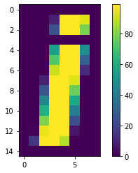
The image displayed is colorful because matplotlib is using the default colormap (a mapping from values in the array to colors). The default colormap in matplotlib is viridis, which maps low numbers to purple and high numbers to yellow. The relationship of numbers to colors can be seen using colorbar.
colormap can be easily changed using the cmap argument.
plt.imshow(X2, cmap='coolwarm')
plt.colorbar();
3-D Surface Plots
Various 3-D plots can be created using matplotlib. 3-D plots are enabled by importing the mplot3d toolkit. Once this submodule is imported, a three-dimensional axes can be created by passing the keyword projection='3d' to any of the normal axes creation. Let's create a 3-D surface plot.
from mpl_toolkits import mplot3d# Make data
X = np.arange(-5, 5, 0.25)
Y = np.arange(-5, 5, 0.25)
X, Y = np.meshgrid(X, Y)
R = np.sqrt(X**2 + Y**2)
Z = np.sin(R)# Plot
fig = plt.figure(figsize=(8,5))
ax = plt.axes(projection='3d')
ax.plot_surface(X, Y, Z, rstride=1, cstride=1,
cmap='coolwarm', edgecolor='none')
ax.set_title('Surface Plot');
Conclusion
In this part of the guide series we introduced NumPy, a foundational package for numerical computing in Python. We discussed how N-dimensional arrays ndarray can be created and then accessed in multiple ways using indexing and slicing. You have seen in detail how universal functions use the concept of Vectorization to perform element-wise operations on arrays. You were also introduced to the basics of plotting arrays.
In the next part of this guide series, you will learn about Introduction to Pandas.
References
[1] Wes McKinney. 2017. Python for Data Analysis: Data Wrangling with Pandas, NumPy, and IPython (2nd. ed.). O'Reilly Media, Inc.
[2] Jake VanderPlas. 2016. Python Data Science Handbook: Essential Tools for Working with Data (1st. ed.). O'Reilly Media, Inc.
[3] Harris, C.R., Millman, K.J., van der Walt, S.J. et al. Array programming with NumPy. Nature 585, 357–362 (2020). https://doi.org/10.1038/s41586-020-2649-2