Introduction
Text classification also known as text tagging or text categorization is the process of assigning tags/labels to unstructured text. Using Natural Language Processing (NLP), text classifiers can automatically analyze text and then assign a set of pre-defined tags or categories based on its content.
As with any other classification problem, text classification can be broadly divided into 2 different categories:
- Multi-class single-label text classification
- Multi-class multi-label text classification
Multi-class single-label text classification
The set of problems where one can associate only a single label to a given input text falls into this category. Take an example of a house address. The address can be associated with a single country. Hence classifying/ tagging a house address to a country is an example of multi-class single-label text classification problem. Other examples include:
- Sentiment Analysis on tweets/movie reviews.
- Classifying emails as Spam vs not Spam
- Language detection from text
Multi-class multi-label text classification
The set of problems where one can associate multiple labels to a given input text falls into this category. Take an example where we are moderating a social media platform by flagging inappropriate user comments and posts. An inappropriate post can fall into multiple categories like toxic, threat, insult, obscene etc. Other examples include:
- Analyze customer support tickets to quickly assign appropriate categories.
- Categorization of News Articles into appropriate topics.
The TextClassifier class in arcgis.learn.text module is based on Hugging Face Transformers library. This library provides transformer models like BERT, RoBERTa, XLM, DistilBert, XLNet etc., for Natural Language Understanding (NLU) with over 32+ pretrained models in 100+ languages.
The transformers are the most latest and advanced models that give the state of the art results for a wide range of tasks such as text / sequence classification, named entity recognition (ner), question answering, machine translation, text summarization, text generation, etc.
Prerequisites
- Data preparation and model training workflows for text classification using
arcgis.learn.textis based on Hugging Face Transformers library. A user can choose an appropriate architecture to train the model. - Refer to the section Install deep learning dependencies of arcgis.learn module for detailed explanation about deep learning dependencies.
- Labeled data: For
TextClassifierto learn, it needs to see examples that have been labeled for all the custom categories that the model is expected to classify an input text into. Head to the Data preparation section to see the supported formats for training data.
Transformer Basics
Transformers in NLP are novel architectures that aims to solve sequence-to-sequence tasks while handling long-range dependencies with ease. The Transformer was proposed in the paper Attention Is All You Need. A transformer consists of an encoding component, a decoding component, and connections between them.

Figure1: A high-level view depicting components of a Transformer [1]
- The Encoding component is a stack of encoders (the paper stacks six of them on top of each other).
- The Decoding component is a stack of decoders of the same number.
The encoders are all identical in structure (yet they do not share weights). Each one is broken down into two sub-layers:
-
Self-Attention Layer
-
Say the following sentence is an input sentence we want to translate:
The animal didn't cross the street because it was too tiredWhat does "it" in this sentence refer to? Is it referring to the street or to the animal? It's a simple question to a human, but not as simple to an algorithm. When the model is processing the word "it", self-attention allow the model to associate "it" with "animal".
-
-
Feed Forward Layer - The outputs of the self-attention layer are fed to a feed-forward neural network.
The decoder has both those layers (self-attention & feed forward layer), but between them is an attention layer (sometimes called encoder-decoder attention) that helps the decoder focus on relevant parts of the input sentence.

Figure2: Different Layers in Transformer's Encoder & Decoder component[1]
To get a more detailed explanation on how attention[2] mechanism works in transformer models visit this page.
An “annotated”[3] version of the paper is also present in the form of a line-by-line implementation of the transformer architecture.
Data preparation
The TextClassifier class in arcgis.learn.text module can consume labeled training data in CSV or TSV file format
There is a slight variation in the way the input data is created for
- Multi-class single-label text classification
- Multi-class multi-label text classification
Sample input data format for Multi-class single-label text classification problem

Sample input data format for Multi-class multi-label text classification problem
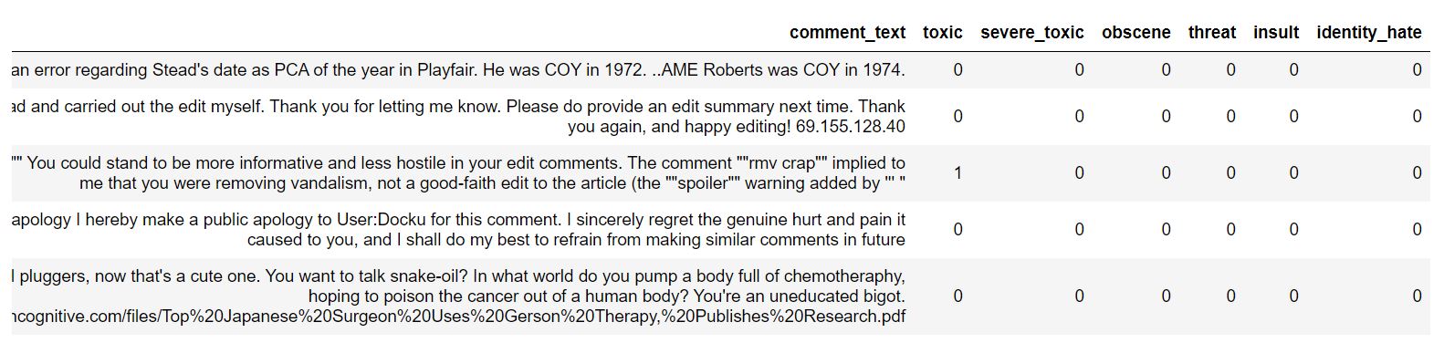
The main difference is that in a Multi-class single-label text classification problem, we have a single target column, but in a Multi-class multi-label text classification problem we have multiple target columns to train the model. The class values are binary(0/1), where the value of 1 represents the presence of a particular class/label for the given training sample and 0 represents the absence of it. In the sample shown above a text can be assigned into 6 different categories toxic, severe_toxic, obscene, threat, insult and identity_hate. A column value of 1 (see row #3) means that the comment/text is labeled as the column name (toxic in this case).
Data preparation involves splitting the data into training and validation sets, creating the necessary data structures for loading data into the model and so on. The prepare_textdata function can directly read the training samples in one of the above specified formats and automate the entire process. While calling this function, the user has to provide the following arguments:
- path - The full directory path where the training file is present
- task - The task for which the dataset is being prepared. The available choice at this point is "classification"
- train_file - The file name containing the training data. Supported file formats/extensions are .csv and .tsv
- text_columns - The column name in the csv/tsv file that will be used as feature.
- label_columns - The list of columns denoting the class label to predict. Provide a list of columns in case of a multi-label classification problem
Some pre-processing functions are also provided like removing HTML tags from the text or removing the URLs from the text. Users can decide if these pre-processing steps are required for their dataset or not.
A note on the dataset
- The data is collected around 2020-05-27 by OpenAddresses.
- The data licenses can be found in
data/country-classifier/LICENSE.txt.
import pandas as pd
from arcgis.learn import prepare_textdata
from arcgis.learn.text import TextClassifier
DATA_ROOT = "data/country_classifier/"data = prepare_textdata(DATA_ROOT, "classification", train_file="house-addresses.csv",
text_columns="Address", label_columns="Country", batch_size=64)print(data.classes)['US', 'BE', 'AU', 'ZA', 'CA', 'BR', 'MX', 'FR', 'JP', 'ES']
The show_batch() method can be used to visualize the training samples, along with labels.
data.show_batch(rows=10)| Address | Country |
|---|---|
| 10, Place Cockerill, 0051, 4000 | BE |
| 547, RUA DIRCEU LOPES, CASA, Pedro Leopoldo, MG, 33600-000 | BR |
| 2, Rue de Ker Izella, Botsorhel, 29650 | FR |
| 168, RUA CORONEL MOREIRA CESAR, APARTAMENTO 402, Niterói, RJ, 24230-062 | BR |
| 732P, CL ARENAL, 33740 | ES |
| 17-9, 高柳新田 | JP |
| S/N, CALLE VENUSTIANO CARRANZA, NICOLÁS BRAVO, Othón P. Blanco, Quintana Roo | MX |
| SN, CALLE FRONTERA, MAZATLÁN, Mazatlán, Sinaloa | MX |
| 41, Oostmallebaan, Zoersel, 2980 | BE |
| SN, RUA ENGENHO PROPRIEDADE, Sirinhaém, PE, 55580-000 | BR |
TextClassifier model
TextClassifier model in arcgis.learn.text is built on top of Hugging Face Transformers library. The model training and inferencing workflow are similar to computer vision models in arcgis.learn.
Run the command below to see which transformer backbones are supported for the classification task.
print(TextClassifier.supported_backbones)['BERT', 'RoBERTa', 'DistilBERT', 'ALBERT', 'FlauBERT', 'CamemBERT', 'XLNet', 'XLM', 'XLM-RoBERTa', 'Bart', 'ELECTRA', 'Longformer', 'MobileBERT']
How to choose an appropriate model for your dataset?
This page mentions different transformers architectures [4] which come in different sizes (model parameters), trained on different languages /corpus, having different attention heads, etc. Not every model can be used for text classification purpose. As of now, there are around 13 models that can be used to perform text classification. These are BERT[5], RoBERTa, DistilBERT, ALBERT, FlauBERT, CamemBERT, XLNet, XLM, XLM-RoBERTa, Bart, ELECTRA, Longformer and MobileBERT
Some consideration has to be made to pick the right transformer architecture for the problem at hand.
- Some models like
BERT,RoBERTa,XLNET,XLM-RoBERTaare highly accurate but at the same time are larger in size. Generating inference from these models is somewhat slow. - If one wishes to sacrifice a little accuracy over a high inferencing and training speed one can go with
DistilBERT. - If the model size is a constraint then one can either choose
ALBERTorMobileBERT. Remember the model performance will not be as great compared to models likeBERT,RoBERTa,XLNET, etc. - If you have a dataset in the French language one can choose from
FlauBERTorCamemBERTas these language model are trained on French text. - When dealing with long sentences/sequences in training data one can choose from
XLNET,Longformer,Bart. - Some models like
XLM,XLM-RoBERTaare multi-lingual models i.e, models trained on multiple languages. If your dataset consists of text in multiple languages you can choose models mentioned in the above link.- The model sizes of these transformer architectures are very large (in GBs).
- They require large memory to fine tune on a particular dataset.
- Due to the large size of these models, inferencing a fined-tuned model will be somewhat slow on CPU.
The HuggingFace Transformers library provides a wide variety of models for each of the backbone listed above. To see the full list visit this link.
- The call to
available_backbone_modelsmethod will list out only a few of the available models for each backbone. - This list is not exhaustive and only contains a subset of the models listed in the link above. This function is created to give a general idea to the user about the available models for a given backbone.
- That being said, the
TextClassifiermodule supports any model from the 13 available backbones. - Some of the Transformer models are quite large due to the high number of training parameters or high number of intermediate layers. Thus large models will have large CPU/GPU memory requirements.
print(TextClassifier.available_backbone_models("xlm-roberta"))('xlm-roberta-base', 'xlm-roberta-large')
Construct the TextClassifier by passing the data and the backbone you have chosen.
The dataset consists of addresses in multiple languages like Japanese, English, French, Spanish, etc. hence we will use a multi-lingual transformer backbone like XLM-RoBERTa to train our model.
model = TextClassifier(data, backbone="xlm-roberta-base")Model training
Finding optimum learning rate
In machine learning, the learning rate[6] is a tuning parameter that determines the step size at each iteration while moving toward a minimum of a loss function, it represents the speed at which a machine learning model "learns"
- If the learning rate is low, then model training will take a lot of time because steps towards the minimum of the loss function are tiny.
- If the learning rate is high, then training may not converge or even diverge. Weight changes can be so big that the optimizer overshoots the minimum and makes the loss worse.
We have to find an optimum learning rate for the dataset we wish to train our model on. To do so we will call the lr_find() method of the model.
Note
- A user is not required to call the
lr_find()method separately. Iflrargument is not provided while calling thefit()method thenlr_find()method is internally called by thefit()method to find the optimal learning rate.
model.lr_find()
0.001445439770745928
Training the model is an iterative process. We can train the model using its fit() method till the validation loss (or error rate) continues to go down with each training pass also known as epoch. This is indicative of the model learning the task.
model.fit(epochs=6, lr=0.001)| epoch | train_loss | valid_loss | accuracy | error_rate | time |
|---|---|---|---|---|---|
| 0 | 0.173400 | 0.111699 | 0.956300 | 0.043700 | 05:24 |
| 1 | 0.062744 | 0.044339 | 0.981100 | 0.018900 | 05:15 |
| 2 | 0.040257 | 0.029966 | 0.986300 | 0.013700 | 05:22 |
| 3 | 0.032077 | 0.024974 | 0.989300 | 0.010700 | 05:32 |
| 4 | 0.030770 | 0.024296 | 0.989800 | 0.010200 | 05:19 |
| 5 | 0.027273 | 0.023898 | 0.990600 | 0.009400 | 05:21 |
Evaluate model performance
model.accuracy()0.9906
Other important metrics to look at are Precision, Recall & F1-measures [7].
Here is a brief description of them:
- Precision - Precision talks about how precise/accurate your model is. Out of those predicted positive, how many of them are actually positive.
- Recall - Recall is the ability of the classifier to find all the positive samples.
- F1 - F1 can be interpreted as a weighted harmonic mean of the precision and recall
To learn more about these metrics one can visit the following link - Precision, Recall & F1 score
To find precision, recall & f1 scores per label/class we will call the model's metrics_per_label() method.
model.metrics_per_label()| Precision_score | Recall_score | F1_score | Support | |
|---|---|---|---|---|
| AU | 1.0000 | 1.0000 | 1.0000 | 929.0 |
| BE | 1.0000 | 1.0000 | 1.0000 | 1043.0 |
| BR | 1.0000 | 1.0000 | 1.0000 | 950.0 |
| CA | 0.9295 | 0.9799 | 0.9541 | 996.0 |
| ES | 1.0000 | 1.0000 | 1.0000 | 982.0 |
| FR | 1.0000 | 1.0000 | 1.0000 | 1009.0 |
| JP | 1.0000 | 0.9990 | 0.9995 | 989.0 |
| MX | 1.0000 | 1.0000 | 1.0000 | 1024.0 |
| US | 0.9803 | 0.9318 | 0.9554 | 1070.0 |
| ZA | 1.0000 | 1.0000 | 1.0000 | 1008.0 |
Validate results
Once we have the trained model, we can see the results to see how it performs.
model.show_results(15)| text | target | prediction |
|---|---|---|
| SN, AVENIDA JOSE MARIA MORELOS Y PAVON OTE., APATZINGÁN DE LA CONSTITUCIÓN, Apatzingán, Michoacán de Ocampo | MX | MX |
| 906, AVENIDA JOSEFA ORTÍZ DE DOMÍNGUEZ, CIUDAD MENDOZA, Camerino Z. Mendoza, Veracruz de Ignacio de la Llave | MX | MX |
| 32, CIRCUITO JOSÉ MARÍA URIARTE, FRACCIONAMIENTO RANCHO ALEGRE, Tlajomulco de Zúñiga, Jalisco | MX | MX |
| SN, ESTRADA SP 250 SENTIDO GRAMADAO, LADO DIREITO FAZENDA SAO RAFAEL CASA 4, São Miguel Arcanjo, SP, 18230-000 | BR | BR |
| SN, CALLE JOSEFA ORTÍZ DE DOMÍNGUEZ, RINCÓN DE BUENA VISTA, Omealca, Veracruz de Ignacio de la Llave | MX | MX |
| SN, CALLE MICHOACAN, DOLORES HIDALGO CUNA DE LA INDEPENDENCIA NACIONAL, Dolores Hidalgo Cuna de la Independencia Nacional, Guanajuato | MX | MX |
| SN, CALLE VERDUZCO, COALCOMÁN DE VÁZQUEZ PALLARES, Coalcomán de Vázquez Pallares, Michoacán de Ocampo | MX | MX |
| 1712, CALLE MÁRTIRES DEL 7 DE ENERO, CIUDAD MENDOZA, Camerino Z. Mendoza, Veracruz de Ignacio de la Llave | MX | MX |
| SN, AVENIDA JACOBO GÁLVEZ, FRACCIONAMIENTO RANCHO ALEGRE, Tlajomulco de Zúñiga, Jalisco | MX | MX |
| SN, ANDADOR MZNA 6 AMP. LOS ROBLES, EL PUEBLITO (CRUCERO NACIONAL), Córdoba, Veracruz de Ignacio de la Llave | MX | MX |
| SN, CALLE SÉPTIMA PONIENTE SUR (EJE VIAL), COMITÁN DE DOMÍNGUEZ, Comitán de Domínguez, Chiapas | MX | MX |
| 18, CALLE FELIPE GORRITI / FELIPE GORRITI KALEA, Pamplona / Iruña, Pamplona / Iruña, Navarra, 31004 | ES | ES |
| SN, RUA X VINTE E SEIS, QUADRA 14 LOTE 35 SALA 3, Aparecida de Goiânia, GO, 74922-680 | BR | BR |
| SN, CALLE NINGUNO, HEROICA CIUDAD DE JUCHITÁN DE ZARAGOZA, Heroica Ciudad de Juchitán de Zaragoza, Oaxaca | MX | MX |
| 1169, RUA DOUTOR ALBUQUERQUE LINS, BLOCO B ANDAR 11 APARTAMENTO 112B, São Paulo, SP, 01203-001 | BR | BR |
Test the model prediction on an input text
text = """1016, 8A, CL RICARDO LEON - SANTA ANA (CARTAGENA), 30319"""
print(model.predict(text))
('1016, 8A, CL RICARDO LEON - SANTA ANA (CARTAGENA), 30319', 'ES', 1.0)
Once you are satisfied with the model, you can save it using the save() method. This creates a Deep Learning Package (DLPK file) that can be used for inferencing on unseen data.
model.save("country-classifier")Computing model metrics...
WindowsPath('models/country-classifier')Model inference
The trained model can be used to classify new text documents using the predict() method. This method accepts a string or a list of strings to predict the labels of these new documents/text.
# Here we are picking addresses from validation dataset, but user can pick/create his/her own list
text_list = data._valid_df.sample(15).Address.values
result = model.predict(text_list)

df = pd.DataFrame(result, columns=["Address", "CountryCode", "Confidence"])

df.style.set_table_styles([dict(selector='th', props=[('text-align', 'left')])])\
.set_properties(**{'text-align': "left"}).hide_index()| Address | CountryCode | Confidence |
|---|---|---|
| 136, AV MARINA ALTA DE LA, 3740 | ES | 0.999972 |
| 3, CL CLOTS DELS, 43791 | ES | 1.000000 |
| FAZENDA LAJEADO, Mimoso do Sul, ES, 29400-000 | BR | 1.000000 |
| 118, CALLE MONTE DE PIEDAD, SAN JUAN DE LOS LAGOS, San Juan de los Lagos, Jalisco | MX | 1.000000 |
| 138A, CALLE EMILIANO ZAPATA, CIUDAD GUZMÁN, Zapotlán el Grande, Jalisco | MX | 1.000000 |
| 28, Rue Gustave Eiffel, Brie-Comte-Robert, 77170 | FR | 1.000000 |
| 19235, AVENUE 6, MADERA, 93637 | US | 0.999995 |
| 2734, CALLE GÓMEZ FARÍAS, GUADALAJARA, Guadalajara, Jalisco | MX | 1.000000 |
| 4237, WHISKEY AVE | CA | 0.542203 |
| 224, SWANSEA ROAD, MOUNT EVELYN, VIC, 3796 | AU | 1.000000 |
| 920, N MARTIN L KING BLVD | US | 0.998366 |
| 13, HOLBERG STREET, MOONEE PONDS, VIC, 3039 | AU | 1.000000 |
| 8, AVENIDA RONCESVALLES / ORREAGA ETORBIDEA, Pamplona / Iruña, Pamplona / Iruña, Navarra, 31002 | ES | 1.000000 |
| 36, Rue Alphonse Hottat, 38, 1050 | BE | 1.000000 |
| SN, CALLE 55 COBA, JOSÉ MARÍA MORELOS, José María Morelos, Quintana Roo | MX | 1.000000 |
References
[2] Attention and its Different Forms
[5] BERT Paper
[6] Learning Rate