The arcgis.raster module contains classes and raster analysis functions for working with raster data and imagery layers.
Raster data is made up of a grid of cells, where each cell or pixel can have a value. Raster data is useful for storing data that varies continuously, as in a satellite image, a surface of chemical concentrations, or an elevation surface.
The Imagerylayer class represents an image service resource as a layer. An ImageryLayer object retrieves and displays data from image services. ImageryLayer allows you to and apply server defined or client-defined rendering rules (e.g. remap, colormap), and mosaic rules.
Accesssing Imagery Layers
Imagery layer items are available as content in the GIS. You can search the GIS for imagery layer items, or get them using their item id:
Searching the GIS for imagery layer items
You can search the GIS for imagery layers by specifying the item type as Imagery Layer:
import arcgis
from arcgis.gis import GIS
from IPython.display import display

gis = GIS()
items = gis.content.search("Landsat 8 Views", item_type="Imagery Layer", max_items=2)for item in items:
display(item)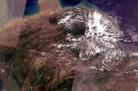
Retrieving Imagery Layer item using item id
Imagery Layers items can be obtained using their item id as well:
l8_views = gis.content.get('4ca13f0e4e29403fa68c46d188c4be73')
l8_views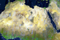
Accessing ImageryLayer from Imagery Layer items
Like other layer based items in the GIS, imagery layer items allow access to the imagery layer through the layers property of the item. Each imagery layer item has one imagery layer instance in it's layers property:
l8_views.layers[<ImageryLayer url:"https://landsat2.arcgis.com/arcgis/rest/services/Landsat8_Views/ImageServer">]
l8_lyr = l8_views.layers[0]
l8_lyr
Creating ImageryLayer from an image service url
ImageryLayer objects can also be constructed from an image service URL using the Service class in the arcgis.layers module:
img_svc_url = 'https://landsat2.arcgis.com/arcgis/rest/services/Landsat8_Views/ImageServer'from arcgis.layers import Servicelandsat_lyr = Service(
url_or_item=img_svc_url
)landsat_lyr
Creating ImageryLayer from secure image services
If the imagery layer is a served by a secure image service, pass in the GIS object to the ImageryLayer constructor to specify the GIS which should be used to connect to the service.
portal = GIS(
    url='https://your_url_to_org/web_adaptor',
    username='your_user',
    password='your_secure_password'
)
secure_url = 'https://your_server:6443/arcgis/rest/services/ImgSrv_Landast_Montana2015/ImageServer'secure_img_lyr = Service(secure_url, portal)secure_img_lyr.url'https://your_server:6443/arcgis/rest/services/ImgSrv_Landast_Montana2015/ImageServer'
Properties of an ImageryLayer object
The properties property on an ImageryLayer object provides a dictionary representation of all its properties. However, you can access individual properties as attributes as well:
landsat_lyr.properties.name'Landsat8_Views'
landsat_lyr.properties['description']'Multispectral Landsat 8 OLI Image Service covering the landmass of the World. This service includes 8-band multispectral scenes, at 30 meter resolution. It can be used for mapping and change detection of agriculture, soils, vegetation health, water-land features and boundary studies. Using on-the-fly processing, the raw DN values are transformed to scaled (0 - 10000) apparent reflectance values and then different service based renderings for band combinations and indices are applied. The service is updated on a daily basis to include the latest best scenes from the USGS.'
The capabilities property is useful to know what kinds of operations can be performed on the imagery layer.
landsat_lyr.properties.capabilities'Image,Metadata,Catalog,Mensuration'
You can access the allowed mosaic methods using the allowedMosaicMethods property.
landsat_lyr.properties.allowedMosaicMethods'ByAttribute,Center,NorthWest,Nadir,LockRaster,None'
Raster Functions
Imagery Layers can be published with raster functions that can be used to change the visualization of the imagery layer using on-the-fly image processing at display resolution. Raster functions are lightweight and process only the pixels visible on your screen, in memory, without creating intermediate files. Raster functions can also be applied at source resolution across the extent of an Imagery Layer using the distributed raster analytics capability provided by Image Server.
Raster Functions are powerful because you can chain them together and apply them on huge rasters and mosaics.
The code below cycles through the raster functions available with the landsat layer:
for fn in landsat_lyr.properties.rasterFunctionInfos:
    print(fn['name'])
Agriculture with DRA Bathymetric with DRA Color Infrared with DRA Geology with DRA Natural Color with DRA Short-wave Infrared with DRA Agriculture Bathymetric Color Infrared Geology Natural Color Short-wave Infrared NDVI Colorized Normalized Difference Moisture Index Colorized NDVI Raw NBR Raw Band 10 Surface Temperature in Fahrenheit Band 11 Surface Temperature in Fahrenheit Band 10 Surface Temperature in Celsius Band 11 Surface Temperature in Celsius None
Visualizing imagery layers
ImageryLayers can be added to the map widget for visualization:
map = gis.map("Pallikaranai")
map
map.content.add(landsat_lyr)Performing on-the-fly image processing using raster functions
The utility of raster functions is better seen when we interactively cycle through these raster functions and apply them to the map, like the code below does. This is using on-the-fly image processing at display resolution to cycle through the various raster functions, and showing how the layer can be visualized using these different raster functions published with the layer:
import time
from arcgis.raster.functions import apply

for fn in landsat_lyr.properties.rasterFunctionInfos:
    print(fn['name'])
    map.content.remove(0)
    map.content.add(apply(landsat_lyr, fn['name']))
    time.sleep(2)
Agriculture with DRA Bathymetric with DRA Color Infrared with DRA Geology with DRA Natural Color with DRA Short-wave Infrared with DRA Agriculture Bathymetric Color Infrared Geology Natural Color Short-wave Infrared NDVI Colorized Normalized Difference Moisture Index Colorized NDVI Raw NBR Raw Band 10 Surface Temperature in Fahrenheit Band 11 Surface Temperature in Fahrenheit Band 10 Surface Temperature in Celsius Band 11 Surface Temperature in Celsius None
Using well-known raster functions
In addition to the raster functions that are published as part of an imagery layer, users can make use of a few well-known raster functions. For instance, in the example below, let us apply an index called NDVI which can be computed using BandArithmetic raster function.
SAVI - The Soil-Adjusted Vegetation Index (SAVI) is a vegetation index that attempts to minimize soil brightness influences using a soil-brightness correction factor. This is often used in arid regions where vegetative cover is low. SAVI is computed as below, where L is the vegetation correction factor and varies from 1 to 0. A value L = 1 is used for no vegetation cover and L=0 for high vegetation cover.
SAVI = ((NIR - Red) / (NIR + Red + L)) x (1 + L)
savi_map = gis.map("Cairo")
savi_map
from arcgis.raster.functions import savi

savi_map.content.add(savi(landsat_lyr, band_indexes="5 4 0.3"))
In the example above, we used one of a 'well-known raster function' BandArithmetic to apply a vegetation index. This index illustrates how the banks and delta of the Nile river appears fertile in a relatively an arid Sahara desert.
Chaining raster functions
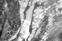
Developers can chaining different raster functions. For instance, the code below is using ExtractBand function to create a [4,5,3] band combination, and applying the Stretch function to get the land-water boundary visualization that makes it easy to see where land is and where water is. Its worth noting that the raster function is applied at display resolution and only for the visible extent using on the fly image processing.
Let us apply this raster function to the imagery layer to visualize the results. The raster function extracts the [4, 5, 3] band combination from Landsat data that makes it easy to visualize where land is and where water is, as seen below:
from arcgis.raster.functions import *

land_water = stretch(extract_band(landsat_lyr, [4, 5, 3]),
                     stretch_type='PercentClip',
                     min_percent=2,
                     max_percent=2,
                     dra=True,
                     gamma=[1, 1, 1])
map2 = gis.map("Pallikaranai")
map2.zoom = 13
map2
map2.content.add(land_water)