Introduction
The World is changing every day and monitoring that change on ground can be a tedious and labor intensive task. so, is there a way to automate it?
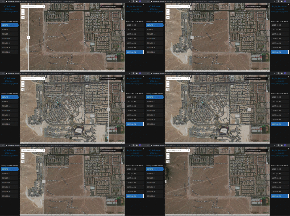
This notebook will walk you through how deep learning can be used to perform change detection using satellite images.
One of the popular models available in the arcgis.learn module of ArcGIS API for Python, ChangeDetector is used to identify areas of persistent change between two different time periods using remotely sensed images. It can help you identify where new buildings have come up for instance. This model is based upon the latest research in deep learning and works well with objects of various sizes.
The ChangeDetector model workflow consists of three parts:
- Preparing the training data,
- training a model
- using the trained model for inferencing.
Let’s first prepare the training data.
Export training data for deep learning
In the cells below, we have provided the input rasters and input mask polygons needed to export training data.
from arcgis.gis import GIS
gis = GIS('home')
input_data = gis.content.get('3ebf8ca5f6c245d69e2e0f4358986ed3')
input_datamask_polygons = gis.content.get('6ee0b48611c44b31b499f6cbe202686f')
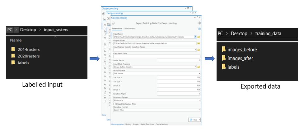
mask_polygonsChangeDetector model requires data in this folder format : images_after, images_before and labels folder. The label indicates where there are changes in the before and after images.
These images are too large to process in the GPU memory for training the model, so we need to create small image chips or tiles. Training data can be exported by using the Export Training Data For Deep Learning tool available in ArcGIS Pro as well as ArcGIS Image Server.
- Input Raster: 2014rasters
- Tile Size X & Tile Size Y: 256
- Stride X & Stride Y: 64
- Meta Data Format: 'Export Tiles'
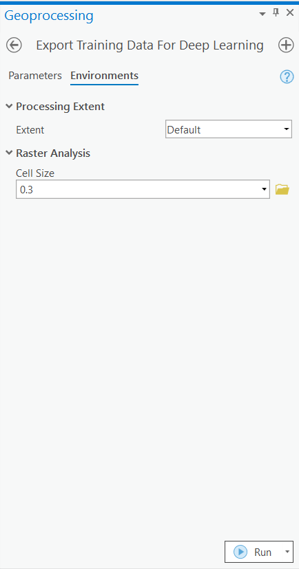
- Environments: 0.3
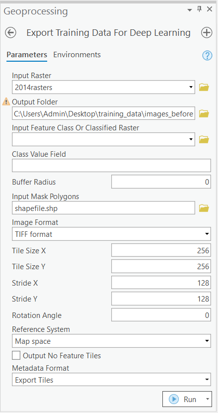
As shown below, the above tool needs to be run thrice each for image before, image after and the change labels in order to create training data.
Model training
This step would be done using jupyter notebook and documentation is available here to install and setup environment.
Necessary imports
import os
from pathlib import Path
from arcgis.learn import prepare_data, ChangeDetector
Get training data
We have already exported the data which can be directly downloaded using the steps below:
training_data = gis.content.get('d284e2083b254f6b8508f9cf41f53713')
training_datafilepath = training_data.download(file_name=training_data.name)import zipfile
with zipfile.ZipFile(filepath, 'r') as zip_ref:
zip_ref.extractall(Path(filepath).parent)data_path = Path(os.path.join(os.path.splitext(filepath)[0]))prepare_data function takes path to training data and creates a fast.ai databunch with specified transformation, batch size, split percentage, etc.
data = prepare_data(data_path,
                    chip_size=256,
                    dataset_type='ChangeDetection',
                    batch_size=4
                   )
Visualize training data
To get a sense of what the training data looks like, use the show_batch() method to randomly pick a few training chips and visualize them. The chips are overlaid with masks representing the building footprints in each image chip.
data.show_batch()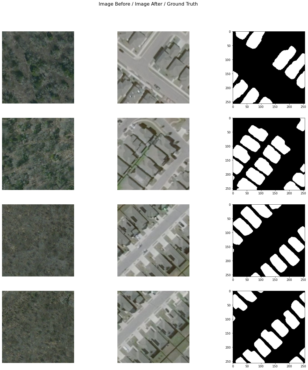
Load model architecture
arcgis.learn provides the ChangeDetector model for identifying areas of persistent change tasks, which is based on a pretrained convnet, like ResNet that acts as the 'backbone'. More details about ChangeDetector can be found here.
cd = ChangeDetector(data, backbone='resnet50')Train the model
Learning rate is one of the most important hyperparameters in model training. We will use the lr_find() method to find an optimum learning rate at which we can train a robust model.
lr = cd.lr_find()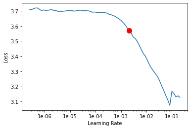
We are using the suggested learning rate above to train the model for 100 epochs.
cd.fit(epochs=100, lr=lr)| epoch | train_loss | valid_loss | precision | recall | f1 | time |
|---|---|---|---|---|---|---|
| 0 | 3.638555 | 3.991394 | 0.000000 | 0.000000 | 0.000000 | 00:20 |
| 1 | 3.582145 | 3.903615 | 0.010081 | 0.001951 | 0.003269 | 00:20 |
| 2 | 3.466630 | 3.788659 | 0.030716 | 0.006106 | 0.007622 | 00:20 |
| 3 | 3.358837 | 3.639781 | 0.178360 | 0.023884 | 0.028300 | 00:20 |
| 4 | 3.222972 | 3.582598 | 0.098645 | 0.022828 | 0.027191 | 00:20 |
| 5 | 3.094626 | 3.514014 | 0.059211 | 0.012516 | 0.015210 | 00:20 |
| 6 | 2.952846 | 3.327957 | 0.121138 | 0.017289 | 0.026279 | 00:20 |
| 7 | 2.781697 | 3.187927 | 0.211084 | 0.011377 | 0.020099 | 00:20 |
| 8 | 2.627799 | 2.962456 | 0.462556 | 0.023596 | 0.042361 | 00:20 |
| 9 | 2.474419 | 2.966377 | 0.374113 | 0.009325 | 0.017576 | 00:20 |
| 10 | 2.326128 | 2.837891 | 0.584811 | 0.013085 | 0.024589 | 00:20 |
| 11 | 2.201696 | 2.678529 | 0.857992 | 0.044994 | 0.079164 | 00:20 |
| 12 | 2.089043 | 2.362821 | 0.832536 | 0.145934 | 0.227257 | 00:20 |
| 13 | 1.969967 | 2.283365 | 0.945265 | 0.189707 | 0.295505 | 00:20 |
| 14 | 1.844372 | 1.952005 | 0.914396 | 0.320796 | 0.458122 | 00:20 |
| 15 | 1.722406 | 1.821877 | 0.942492 | 0.346117 | 0.492069 | 00:20 |
| 16 | 1.619969 | 1.715959 | 0.916230 | 0.392046 | 0.531676 | 00:20 |
| 17 | 1.528037 | 1.713027 | 0.926809 | 0.383866 | 0.532530 | 00:20 |
| 18 | 1.448876 | 1.704992 | 0.923534 | 0.394154 | 0.544590 | 00:20 |
| 19 | 1.376549 | 1.639403 | 0.910712 | 0.426527 | 0.574423 | 00:20 |
| 20 | 1.307974 | 1.650538 | 0.957250 | 0.413184 | 0.570541 | 00:20 |
| 21 | 1.239900 | 1.557845 | 0.938700 | 0.450939 | 0.603749 | 00:20 |
| 22 | 1.189204 | 1.504176 | 0.919200 | 0.470804 | 0.616889 | 00:20 |
| 23 | 1.133861 | 1.335776 | 0.885409 | 0.546320 | 0.670734 | 00:20 |
| 24 | 1.081192 | 1.195659 | 0.926701 | 0.592452 | 0.720968 | 00:20 |
| 25 | 1.026258 | 1.117100 | 0.927687 | 0.622400 | 0.743564 | 00:20 |
| 26 | 0.967815 | 1.111288 | 0.929599 | 0.624123 | 0.744089 | 00:20 |
| 27 | 0.913346 | 1.236537 | 0.932294 | 0.578853 | 0.711762 | 00:20 |
| 28 | 0.862091 | 1.123269 | 0.942785 | 0.622289 | 0.747705 | 00:20 |
| 29 | 0.813487 | 0.978635 | 0.919088 | 0.683585 | 0.781774 | 00:20 |
| 30 | 0.767492 | 0.992773 | 0.945853 | 0.672112 | 0.784134 | 00:20 |
| 31 | 0.730505 | 0.918134 | 0.940509 | 0.704169 | 0.804023 | 00:20 |
| 32 | 0.690950 | 0.905217 | 0.926857 | 0.719895 | 0.808600 | 00:20 |
| 33 | 0.657039 | 0.794999 | 0.925516 | 0.760522 | 0.833842 | 00:20 |
| 34 | 0.630016 | 0.867078 | 0.947797 | 0.731603 | 0.824432 | 00:20 |
| 35 | 0.601195 | 0.699993 | 0.920142 | 0.795124 | 0.852049 | 00:20 |
| 36 | 0.576520 | 0.644506 | 0.915747 | 0.819673 | 0.864064 | 00:20 |
| 37 | 0.555032 | 0.733163 | 0.944261 | 0.780036 | 0.853382 | 00:20 |
| 38 | 0.538826 | 0.659537 | 0.919398 | 0.821423 | 0.866999 | 00:21 |
| 39 | 0.520452 | 0.760795 | 0.944995 | 0.780005 | 0.853581 | 00:20 |
| 40 | 0.512040 | 0.604587 | 0.892046 | 0.837553 | 0.862926 | 00:20 |
| 41 | 0.504215 | 0.771875 | 0.941343 | 0.768384 | 0.844560 | 00:20 |
| 42 | 0.491912 | 0.794373 | 0.949777 | 0.766483 | 0.847167 | 00:21 |
| 43 | 0.478684 | 0.706338 | 0.942926 | 0.800782 | 0.865408 | 00:20 |
| 44 | 0.467712 | 0.569906 | 0.926719 | 0.846304 | 0.884119 | 00:20 |
| 45 | 0.456967 | 0.873639 | 0.963469 | 0.740113 | 0.835746 | 00:20 |
| 46 | 0.447868 | 0.843372 | 0.936705 | 0.749807 | 0.830982 | 00:20 |
| 47 | 0.440795 | 0.720638 | 0.943460 | 0.796371 | 0.862751 | 00:20 |
| 48 | 0.437912 | 0.689829 | 0.939067 | 0.798697 | 0.861709 | 00:20 |
| 49 | 0.433079 | 0.793026 | 0.944043 | 0.761286 | 0.841921 | 00:20 |
| 50 | 0.429685 | 0.753005 | 0.951377 | 0.776167 | 0.853922 | 00:20 |
| 51 | 0.422348 | 1.080390 | 0.977777 | 0.641748 | 0.771623 | 00:20 |
| 52 | 0.418187 | 0.869561 | 0.966335 | 0.730030 | 0.830743 | 00:20 |
| 53 | 0.412941 | 0.965646 | 0.970714 | 0.700501 | 0.812416 | 00:20 |
| 54 | 0.406895 | 0.795781 | 0.970092 | 0.766602 | 0.855860 | 00:20 |
| 55 | 0.405798 | 0.833027 | 0.958539 | 0.739912 | 0.833417 | 00:20 |
| 56 | 0.402146 | 1.052749 | 0.979980 | 0.654134 | 0.781858 | 00:20 |
| 57 | 0.397604 | 0.894821 | 0.964845 | 0.729775 | 0.829408 | 00:20 |
| 58 | 0.395370 | 0.959887 | 0.959718 | 0.705723 | 0.811772 | 00:20 |
| 59 | 0.390840 | 1.008945 | 0.978121 | 0.675790 | 0.797390 | 00:20 |
| 60 | 0.386628 | 0.902825 | 0.957737 | 0.728781 | 0.826430 | 00:20 |
| 61 | 0.385515 | 0.834128 | 0.964658 | 0.755774 | 0.846767 | 00:20 |
| 62 | 0.382837 | 0.999641 | 0.979129 | 0.681938 | 0.802178 | 00:20 |
| 63 | 0.379209 | 0.930604 | 0.968249 | 0.707038 | 0.815698 | 00:20 |
| 64 | 0.377985 | 1.149386 | 0.980999 | 0.614413 | 0.753061 | 00:20 |
| 65 | 0.374265 | 1.141354 | 0.977268 | 0.622048 | 0.757125 | 00:20 |
| 66 | 0.373087 | 0.997541 | 0.975062 | 0.683849 | 0.801910 | 00:20 |
| 67 | 0.369995 | 0.965105 | 0.977323 | 0.694194 | 0.810141 | 00:20 |
| 68 | 0.368643 | 0.965632 | 0.975883 | 0.695690 | 0.810604 | 00:20 |
| 69 | 0.367586 | 1.029196 | 0.983688 | 0.667932 | 0.793804 | 00:20 |
| 70 | 0.363348 | 1.103462 | 0.981277 | 0.634739 | 0.768536 | 00:20 |
| 71 | 0.362918 | 1.136731 | 0.982168 | 0.619785 | 0.757631 | 00:20 |
| 72 | 0.360772 | 1.250651 | 0.982184 | 0.566397 | 0.714903 | 00:20 |
| 73 | 0.361154 | 1.095196 | 0.982624 | 0.634577 | 0.768156 | 00:20 |
| 74 | 0.357480 | 1.169230 | 0.982301 | 0.601907 | 0.742707 | 00:20 |
| 75 | 0.354970 | 1.243248 | 0.986144 | 0.565308 | 0.714099 | 00:20 |
| 76 | 0.353663 | 1.258047 | 0.986308 | 0.557171 | 0.707525 | 00:20 |
| 77 | 0.352631 | 1.169211 | 0.981529 | 0.604592 | 0.744274 | 00:20 |
| 78 | 0.352312 | 1.138829 | 0.985036 | 0.614892 | 0.753574 | 00:20 |
| 79 | 0.349714 | 1.154210 | 0.985081 | 0.607603 | 0.748027 | 00:20 |
| 80 | 0.348625 | 1.168601 | 0.984847 | 0.598727 | 0.740922 | 00:20 |
| 81 | 0.348815 | 1.200720 | 0.983323 | 0.587594 | 0.731428 | 00:20 |
| 82 | 0.347588 | 1.120581 | 0.983028 | 0.622989 | 0.759640 | 00:20 |
| 83 | 0.345640 | 1.198889 | 0.986434 | 0.583340 | 0.729115 | 00:20 |
| 84 | 0.344555 | 1.246538 | 0.986628 | 0.564164 | 0.713712 | 00:20 |
| 85 | 0.346326 | 1.176782 | 0.985689 | 0.595028 | 0.738459 | 00:20 |
| 86 | 0.345176 | 1.217701 | 0.985982 | 0.577031 | 0.724172 | 00:20 |
| 87 | 0.342948 | 1.259189 | 0.986295 | 0.558396 | 0.708423 | 00:20 |
| 88 | 0.342329 | 1.267915 | 0.988048 | 0.552718 | 0.704447 | 00:20 |
| 89 | 0.342835 | 1.297185 | 0.985551 | 0.541281 | 0.694016 | 00:20 |
| 90 | 0.343246 | 1.235277 | 0.987263 | 0.567947 | 0.717025 | 00:20 |
| 91 | 0.344547 | 1.219906 | 0.984894 | 0.576465 | 0.723358 | 00:20 |
| 92 | 0.343386 | 1.182762 | 0.984720 | 0.594058 | 0.737606 | 00:20 |
| 93 | 0.343103 | 1.226689 | 0.985229 | 0.572633 | 0.720289 | 00:20 |
| 94 | 0.343583 | 1.169614 | 0.985558 | 0.601031 | 0.743548 | 00:20 |
| 95 | 0.342515 | 1.213448 | 0.984735 | 0.580992 | 0.727087 | 00:20 |
| 96 | 0.342756 | 1.156660 | 0.983209 | 0.608391 | 0.748602 | 00:20 |
| 97 | 0.343446 | 1.192447 | 0.984951 | 0.588587 | 0.733259 | 00:20 |
| 98 | 0.343412 | 1.214610 | 0.982924 | 0.579534 | 0.725373 | 00:20 |
| 99 | 0.342311 | 1.163522 | 0.983879 | 0.604465 | 0.745752 | 00:20 |
We have further trained the model for 100 more epochs to improve model performance. For the sake of time, the cell below is commented out.
# cd.fit(100)Visualize detected changes
It's a good practice to see results of the model viz-a-viz ground truth. The code below picks random samples and shows us ground truth and model predictions, side by side. This enables us to preview the results of the model within the notebook.
cd.show_results(rows=8) 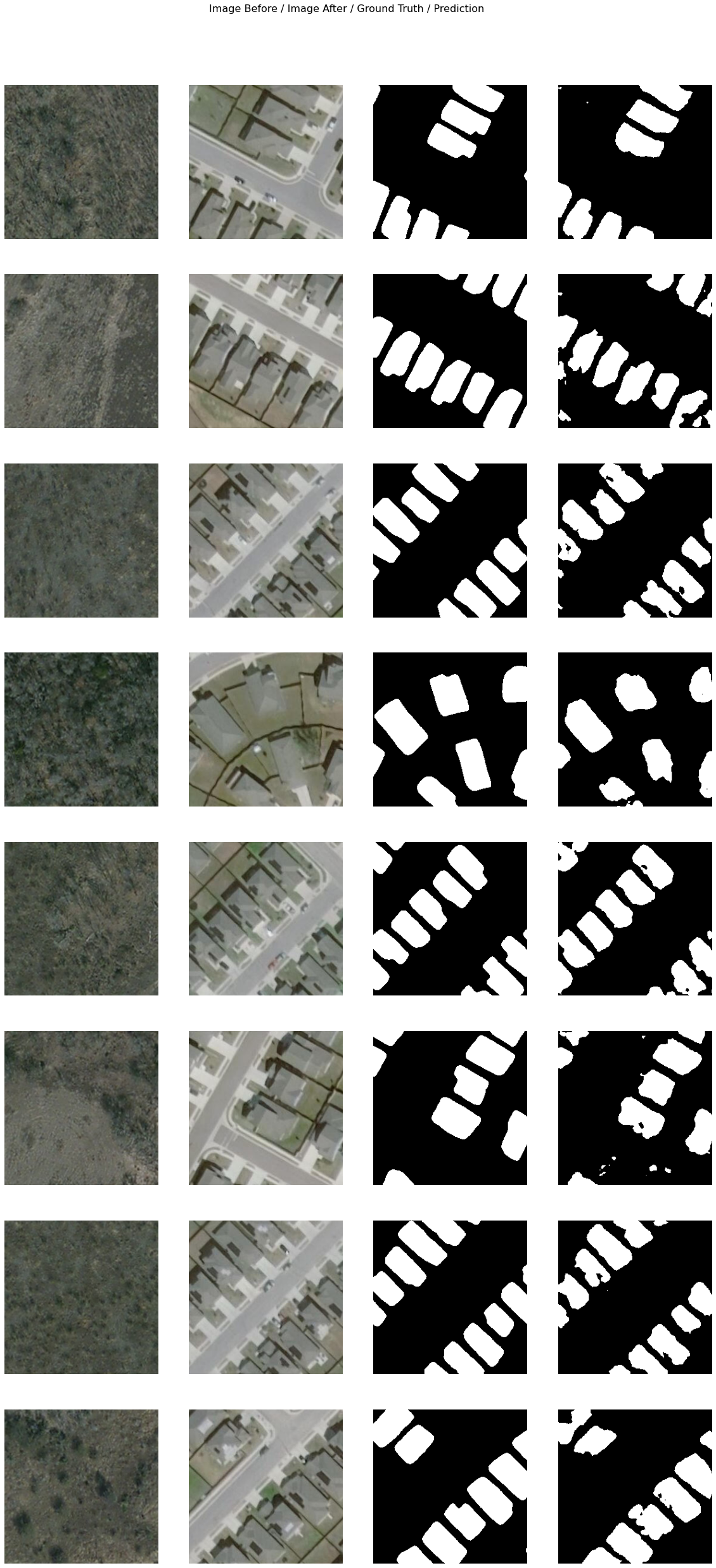
Evaluate model performance
As we have 2 classes for this change detection task, we need to do accuracy assessment for each of those. For that ArcGIS API for Python provides precision_recall_score function that will calculate precision and recall for each class.
cd.precision_recall_score()| NoChange | Change | |
|---|---|---|
| precision | 0.936954 | 0.926067 |
| recall | 0.970100 | 0.848920 |
| f1 | 0.953147 | 0.885244 |
Save model
We will save the model which we trained as a 'Deep Learning Package' ('.dlpk' format). Deep Learning package is the standard format used to deploy deep learning models on the ArcGIS platform.
We will use the save() method to save the trained model. By default, it will be saved to the 'models' sub-folder within our training data folder.
cd.save('change_detection_model_e200')Model inference
Using predict function, we can apply the trained model on a test image/area to detect changes that occurred in the satellite images during two different time periods.
inference_data = gis.content.get('6b32a534228b44b284c14e75b3d3f5f5')
inference_datatest_path = inference_data.download(file_name=inference_data.name)import zipfile
with zipfile.ZipFile(test_path, 'r') as zip_ref:
zip_ref.extractall(Path(test_path).parent)test_images = Path(os.path.join(os.path.splitext(test_path)[0]))before_img = os.path.join(test_images, 'before.tif')
after_img = os.path.join(test_images, 'after.tif')The predict function takes in before and after image path as required variables. You can optionally pass visualize=True if you want to see the results in the notebook. Additionally, you can pass save=True function in order to save the image to the local disk.
cd.predict(before_image=before_img,
           after_image=after_img,
           visualize=True)
tensor([[[0, 0, 0, ..., 0, 0, 0],
[0, 0, 0, ..., 0, 0, 0],
[0, 0, 0, ..., 0, 0, 0],
...,
[0, 0, 0, ..., 0, 0, 0],
[0, 0, 0, ..., 0, 0, 0],
[0, 0, 0, ..., 0, 0, 0]]])
Conclusion
In this notebook, we learned how to solve various problems like identifying new construction. The same workflow can also be used to find out which new roads have come up in the past five years for instance. With just some labeled data and with little to no human involvement by using deep learning, we can now perform change detection using satellite images.

