Introduction
Recently, there has been a great emphasis on reducing the carbon footprint of our cities by moving away from fossil fuels to renewable energy sources. City governments across the world, in this case the City of Calgary, Canada, are leading this change by becoming energy independent through solar power plants, either implemented on rooftops or within city utility sites.
This notebook aims to further aid this move to renewable solar energy by predicting the annual solar energy likely to be generated by a solar power station through local weather information and site characteristics. The hypothesis proposed by this notebook is that various weather parameters, such as temperature, wind speed, vapor pressure, solar radiation, day length, precipitation, snowfall, along with the altitude of a solar power station site, will impact the daily generation of solar energy.
Accordingly, these variables are used to train a model on actual solar power generated by solar power stations located in Calgary. This trained model will then be used to predict solar generation from potential solar power plant sites. Beyond the weather and altitude variables, the total energy generated from a solar station will also depend on the capacity of that station. For instance, a 100kwp solar plant will generate more energy than a 50kwp plant, and the final output will therefore also take into consideration the capacity of each solar power plant.
Imports
%matplotlib inline
import matplotlib.pyplot as plt

import pandas as pd
from pandas import read_csv
from datetime import datetime
from IPython.display import Image, HTML

from sklearn.pipeline import make_pipeline
from sklearn.preprocessing import Normalizer
from sklearn.preprocessing import MinMaxScaler
from sklearn.compose import make_column_transformer
from sklearn.metrics import r2_score

import arcgis
from arcgis.gis import GIS
from arcgis.learn import FullyConnectedNetwork, MLModel, prepare_tabulardata
Connecting to ArcGIS
gis = GIS('home')Accessing & Visualizing datasets
The primary data used for this sample are as follows:
Out of the several solar photovoltaic power plants in the City of Calgary, 11 were selected for the study. The dataset contains two components:
1) Daily solar energy production for each power plant from September 2015 to December 2019.
2) Corresponding daily weather measurements for the given sites.
The datasets were obtained from multiple sources, as mentioned here (Data resources), and preprocessed to obtain the main dataset used in this sample. Two feature layers were subsequently created from this dataset, one dataset for training and the other for validating.
Training Set
The training dataset consists of data from 10 solar sites for training the model. The feature layer containing the data is accessed here from Arcgis portal and visualized as follows:
# Access Solar Dataset feature layer for Training, without the Southland Solar Plant which is hold out for validation
calgary_no_southland_solar = gis.content.get('adaead8cb3174ac6a89f0c14ae70aadd')
calgary_no_southland_solar
# Access the layer from the feature layer
calgary_no_southland_solar_layer = calgary_no_southland_solar.layers[0]
# Plot location of the 10 Solar sites in Calgary to be used for training
m1 = gis.map('calgary', zoomlevel=10)
m1.add_layer(calgary_no_southland_solar_layer)
m1
The map above shows the 10 power plant locations that are used for collecting the training data.
# Visualize the dataframe
calgary_no_southland_solar_layer_sdf = calgary_no_southland_solar_layer.query().sdf
calgary_no_southland_solar_layer_sdf=calgary_no_southland_solar_layer_sdf[['FID','date','ID','solar_plan','altitude_m',
                                                                           'latitude','longitude','wind_speed','dayl__s_',
                                                                           'prcp__mm_d','srad__W_m_','swe__kg_m_', 'tmax__deg',
                                                                           'tmin__deg','vp__Pa_','kWh_filled','capacity_f',
                                                                           'SHAPE']]
calgary_no_southland_solar_layer_sdf.head()| FID | date | ID | solar_plan | altitude_m | latitude | longitude | wind_speed | dayl__s_ | prcp__mm_d | srad__W_m_ | swe__kg_m_ | tmax__deg | tmin__deg | vp__Pa_ | kWh_filled | capacity_f | SHAPE | |
|---|---|---|---|---|---|---|---|---|---|---|---|---|---|---|---|---|---|---|
| 0 | 1 | 2017-12-24 | 355827 | Glenmore Water Treatment Plant | 1095 | 51.003078 | -114.100571 | 7.204670 | 27648.0 | 1 | 108.800003 | 12 | -10.5 | -21.0 | 120 | 1.242357 | 0.000177 | {"x": -12701617.407282012, "y": 6621838.159138... |
| 1 | 2 | 2017-12-25 | 355827 | Glenmore Water Treatment Plant | 1095 | 51.003078 | -114.100571 | 3.385235 | 27648.0 | 1 | 115.199997 | 12 | -18.0 | -29.5 | 40 | 2.477714 | 0.000354 | {"x": -12701617.407282012, "y": 6621838.159138... |
| 2 | 3 | 2017-12-26 | 355827 | Glenmore Water Treatment Plant | 1095 | 51.003078 | -114.100571 | 5.076316 | 27648.0 | 0 | 118.400002 | 12 | -20.0 | -32.0 | 40 | 3.713071 | 0.000530 | {"x": -12701617.407282012, "y": 6621838.159138... |
| 3 | 4 | 2017-12-27 | 355827 | Glenmore Water Treatment Plant | 1095 | 51.003078 | -114.100571 | 5.617623 | 27648.0 | 0 | 96.000000 | 12 | -18.0 | -26.5 | 80 | 4.948429 | 0.000707 | {"x": -12701617.407282012, "y": 6621838.159138... |
| 4 | 5 | 2017-12-28 | 355827 | Glenmore Water Treatment Plant | 1095 | 51.003078 | -114.100571 | 2.561512 | 27648.0 | 0 | 118.400002 | 12 | -17.0 | -28.5 | 40 | 6.183786 | 0.000883 | {"x": -12701617.407282012, "y": 6621838.159138... |
In the table above, each row represents each individual day from September 2015 to December 2019, with the corresponding date shown in the field named date and the name of the solar site in the field named solar_plan.
The primary information consists of the daily generation of energy in kilowatt-hour(KWh) given here in the field name kWh_filled for each of the selected 10 solar photovoltaic power plants in the City of Calgary. The field capacity_f indicates the capacity factor, which is obtained after normalizing the kWh_filled by the peak capacity of each solar photovoltaic sites, and will be used here as the dependent variable.
In addition, it also contains data about weather variables for each day for the related solar plant, all of which, except wind speed, were obtained from MODIS, Daymet observations. These variables are as follows:
- wind_speed : wind speed(m/sec)
- dayl_s : Day length (sec/day)
- prcp__mm_d : Precipitation (mm/day)
- srad_W_m : Shortwave radiation (W/m^2)
- swe_kg_m : Snow water equivalent (kg/m^2)
- tmax__deg : Maximum air temperature (degrees C)
- tmin__deg : Minimum air temperature (degrees C)
- vp_Pa : Water vapor pressure (Pa)
To understand the distribution of the variables over the last few years and their respective relationship with the dependent variable of daily energy produced for a station, data from one of the stations is plotted as follows:
# plot and Visualize the variables from the training set for one solar station - Hillhurst Sunnyside Community Association
hillhurst_solar = calgary_no_southland_solar_layer_sdf[calgary_no_southland_solar_layer_sdf['solar_plan']=='Hillhurst Sunnyside Community Association'].copy()
hillhurst_datetime = hillhurst_solar.set_index(hillhurst_solar['date'])
hillhurst_datetime = hillhurst_datetime.sort_index()
for i in range(7,hillhurst_datetime.shape[1]-1):
        plt.figure(figsize=(20,3))
        plt.title(hillhurst_datetime.columns[i])
        plt.plot(hillhurst_datetime[hillhurst_datetime.columns[i]])
        plt.show()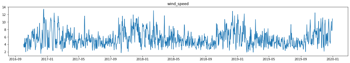
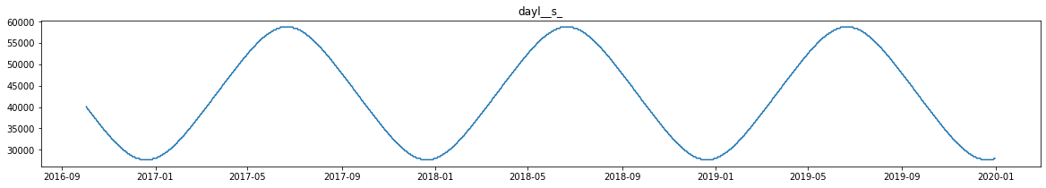
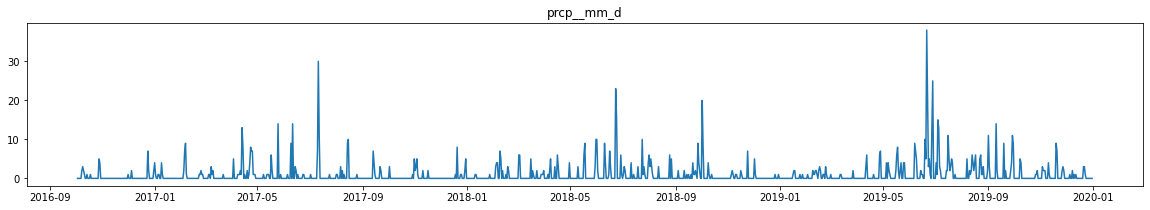
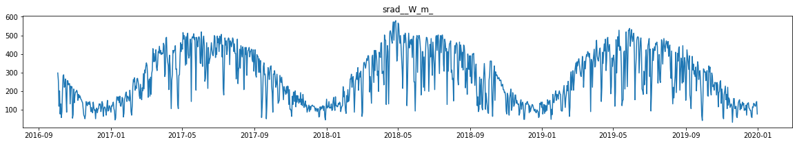
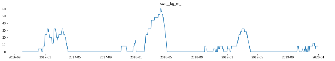
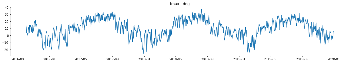
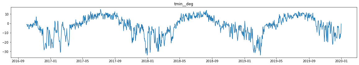
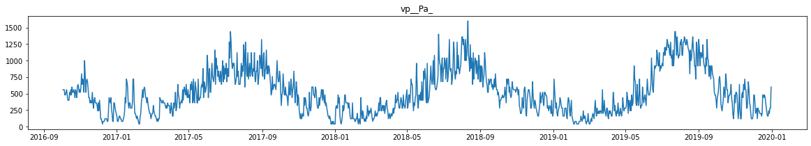
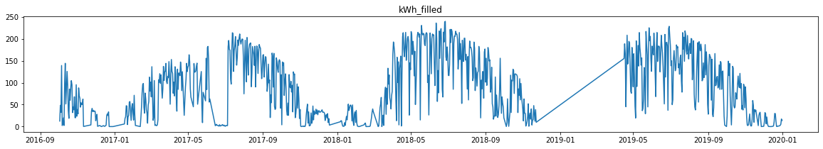
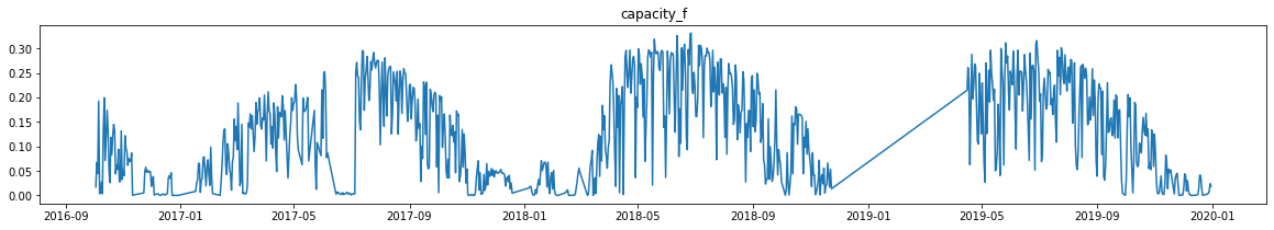
In the plots above, it can be seen that each of the variables has a high seasonality, and it seems that there is a relationship between the dependent variable kWh_filled and the explanatory variables. As such, a correlation plot should be created to check the correlation between the variables.
# checking the correlation matrix between the predictors and the dependent variable of capacity_factor
corr_test = calgary_no_southland_solar_layer_sdf.drop(['FID','date','ID','latitude','longitude','solar_plan','kWh_filled'], axis=1)
corr = corr_test.corr()
corr.style.background_gradient(cmap='Greens').set_precision(2)| altitude_m | wind_speed | dayl__s_ | prcp__mm_d | srad__W_m_ | swe__kg_m_ | tmax__deg | tmin__deg | vp__Pa_ | capacity_f | |
|---|---|---|---|---|---|---|---|---|---|---|
| altitude_m | 1.00 | -0.01 | 0.04 | 0.01 | 0.03 | 0.02 | 0.02 | 0.02 | 0.02 | 0.03 |
| wind_speed | -0.01 | 1.00 | -0.41 | -0.17 | -0.26 | 0.02 | -0.03 | -0.06 | -0.13 | -0.24 |
| dayl__s_ | 0.04 | -0.41 | 1.00 | 0.20 | 0.78 | -0.18 | 0.72 | 0.73 | 0.60 | 0.77 |
| prcp__mm_d | 0.01 | -0.17 | 0.20 | 1.00 | -0.18 | -0.07 | -0.03 | 0.10 | 0.20 | -0.04 |
| srad__W_m_ | 0.03 | -0.26 | 0.78 | -0.18 | 1.00 | 0.04 | 0.69 | 0.50 | 0.28 | 0.82 |
| swe__kg_m_ | 0.02 | 0.02 | -0.18 | -0.07 | 0.04 | 1.00 | -0.45 | -0.48 | -0.46 | -0.19 |
| tmax__deg | 0.02 | -0.03 | 0.72 | -0.03 | 0.69 | -0.45 | 1.00 | 0.93 | 0.75 | 0.75 |
| tmin__deg | 0.02 | -0.06 | 0.73 | 0.10 | 0.50 | -0.48 | 0.93 | 1.00 | 0.85 | 0.65 |
| vp__Pa_ | 0.02 | -0.13 | 0.60 | 0.20 | 0.28 | -0.46 | 0.75 | 0.85 | 1.00 | 0.45 |
| capacity_f | 0.03 | -0.24 | 0.77 | -0.04 | 0.82 | -0.19 | 0.75 | 0.65 | 0.45 | 1.00 |
The resulting correlation plot shows that the variable of shortwave radiation per meter square (srad_W_m) has the largest correlation with the dependent variable of total solar energy produced expressed in terms of capacity factor(capacity_f). This is followed by the variable of day length(dayl_s), as longer days are likely to produce more solar energy. These two are closely followed by max(tmax__deg) and min(tmin__deg) daily temperatures, and lastly the remaining variables with weaker correlation values.
Validation Set
The validation set consists of daily solar generation data from September 2015 to December 2019 for one solar site, known as Southland Leisure Centre, and will be used to validate the trained model.
# Access the Southland Solar Plant Dataset feature layer for validation
southland_solar = gis.content.get('af78423949b94c1783fa43d707df6d45')
southland_solar
# Access the layer from the feature layer
southland_solar_layer = southland_solar.layers[0]
# Plot location of the Southalnd Solar site in Calgary to be used for validation
m1 = gis.map('calgary', zoomlevel=10)
m1.add_layer(southland_solar_layer)
m1
# visualize the southland dataframe here
southland_solar_layer_sdf = southland_solar_layer.query().sdf
southland_solar_layer_sdf.head(2)| FID | Field1 | ID | solar_plan | altitude_m | latitude | longitude | wind_speed | dayl__s_ | prcp__mm_d | ... | tmin__deg | vp__Pa_ | kWh_filled | capacity_f | GlobalID | CreationDate | Creator | EditDate | Editor | SHAPE | |
|---|---|---|---|---|---|---|---|---|---|---|---|---|---|---|---|---|---|---|---|---|---|
| 0 | 1 | 2019-10-03 | 164440 | Southland Leisure Centre | 1100 | 50.962485 | -114.108472 | 5.332239 | 40089.601562 | 0 | ... | -3.0 | 480 | 309.644 | 0.084326 | e9b0f671-d6ba-4560-b912-d635a0a129f8 | 2020-04-27 11:58:02.992000103 | arcgis_python | 2020-04-27 11:58:02.992000103 | arcgis_python | {"x": -12702497.020502415, "y": 6614660.374377... |
| 1 | 2 | 2019-10-04 | 164440 | Southland Leisure Centre | 1100 | 50.962485 | -114.108472 | 6.304829 | 40089.601562 | 0 | ... | -1.0 | 560 | 679.785 | 0.185127 | 7bde5210-a8c2-4731-9c23-e5f77c1ebc56 | 2020-04-27 11:58:02.992000103 | arcgis_python | 2020-04-27 11:58:02.992000103 | arcgis_python | {"x": -12702497.020502415, "y": 6614660.374377... |
2 rows × 23 columns
# check the total number of samples
southland_solar_layer_sdf.shape
(1590, 23)
Model Building
Once the training and the validation dataset have been processed and analyzed, they are ready to be used for modeling.
In this sample, two methods are used for modeling:
1) FullyConnectedNetwork - First a deep learning framework called FullyConnectedNetwork, available in the arcgis.learn module in ArcGIS API for Python, is used.
2) MLModel - In the second method, a regression model from scikit-learn is implemented via the MLModel framework in arcgis.learn. This framework can deploy any regression or classification model from the library by passing the name of the algorithm and its relevant parameters as keyword arguments.
Finally, performance between the two methods will be compared in terms of model training and validation accuracy.
Further details on FullyConnectedNetwork & MLModel are available here in the Deep Learning with ArcGIS section.
1 — FullyConnectedNetwork
This is an Artificial Neural Network model from the arcgis.learn module, which is used here for modeling.
Data Preprocessing
First, a list is made that consists of the feature data that will be used for predicting daily solar energy generation. By default, it will receive continuous variables, and in the case of categorical variables, the True value should be passed inside a tuple along with the variable. In this example, all of the variables are continuous.
# Here a list is created naming all fields containing the predictors from the input feature layer
X = ['altitude_m', 'wind_speed', 'dayl__s_', 'prcp__mm_d','srad__W_m_','swe__kg_m_','tmax__deg','tmin__deg','vp__Pa_']
# importing the libraries from arcgis.learn for data preprocessing
from arcgis.learn import prepare_tabulardataOnce the explanatory variables are identified, the main preprocessing of the data is carried out by the prepare_tabulardata method from the arcgis.learn module in the ArcGIS API for Python. This function will take either a feature layer or a spatial dataframe containing the dataset as input and will return a TabularDataObject that can be fed into the model.
The input parameters required for the tool are:
- input_features : feature layer or spatial dataframe containing the primary dataset
- variable_predict : field name containing the y-variable from the input feature layer/dataframe
- explanatory_variables : list of the field names as 2-sized tuples containing the explanatory variables as mentioned above
# precrocessing data using prepare data method - it handles imputing missing values, normalization and train-test split
data = prepare_tabulardata(calgary_no_southland_solar_layer,
                           'capacity_f',
                           explanatory_variables=X)
# visualizing the prepared data
data.show_batch()| altitude_m | capacity_f | dayl__s_ | prcp__mm_d | srad__W_m_ | swe__kg_m_ | tmax__deg | tmin__deg | vp__Pa_ | wind_speed | |
|---|---|---|---|---|---|---|---|---|---|---|
| 146 | 1095 | 0.008051 | 38707.199219 | 0 | 329.600006 | 8 | 3.0 | -13.5 | 200 | 4.242083 |
| 170 | 1095 | 0.025921 | 33177.601562 | 3 | 70.400002 | 0 | 3.5 | -2.5 | 520 | 5.934033 |
| 391 | 1095 | 0.273637 | 57715.199219 | 0 | 515.200012 | 0 | 26.5 | 4.5 | 480 | 6.532143 |
| 522 | 1095 | 0.016343 | 32140.800781 | 0 | 147.199997 | 0 | -11.5 | -20.0 | 120 | 4.157886 |
| 825 | 1095 | 0.019354 | 29376.000000 | 0 | 102.400002 | 4 | 10.0 | 1.5 | 680 | 6.422836 |
| ... | ... | ... | ... | ... | ... | ... | ... | ... | ... | ... |
| 8390 | 1051 | 0.285307 | 56332.800781 | 0 | 460.799988 | 0 | 27.0 | 8.5 | 520 | 3.335872 |
| 8460 | 1051 | 0.233103 | 54604.800781 | 4 | 300.799988 | 0 | 26.5 | 10.0 | 1200 | 3.828789 |
| 8777 | 1051 | 0.285116 | 57369.601562 | 0 | 537.599976 | 0 | 27.5 | 5.5 | 320 | 4.703076 |
| 9035 | 1096 | 0.002692 | 27993.599609 | 0 | 134.399994 | 0 | -5.5 | -30.0 | 40 | 8.036874 |
| 9056 | 1096 | 0.122572 | 30412.800781 | 0 | 121.599998 | 0 | 4.5 | -6.0 | 400 | 7.787962 |
64 rows × 10 columns
Model Initialization
Once the data has been prepared by the prepare_tabulardata method, it is ready to be passed to the ANN for training. First, the ANN, known as FullyConnectedNetwork, is imported from arcgis.learn and initialized as follows:
# importing the model from arcgis.learn
from arcgis.learn import FullyConnectedNetwork
# Initialize the model with the data where the weights are randomly allocated
fcn = FullyConnectedNetwork(data)Learning Rate Search
# searching for an optimal learning rate using the lr_find for passing it to the final model fitting
fcn.lr_find()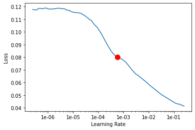
0.0005754399373371565
Here the suggested learning rate by the lr_find method is around 0.0005754. The automatic lr_finder will take a conservative estimate of the learning rate, but some experts can interpret the graph more appropriately and find a better learning rate to be used for final training of the model.
Model Training
Finally, the model is now ready for training. To train the model, the model.fit is called and provided with the number of epochs for training and the estimated learning rate suggested by lr_find in the previous step:
# the model is trained for 100 epochs
fcn.fit(100,0.0005754399373371565)| epoch | train_loss | valid_loss | time |
|---|---|---|---|
| 0 | 0.011153 | 0.004776 | 00:01 |
| 1 | 0.004083 | 0.003175 | 00:01 |
| 2 | 0.002893 | 0.002665 | 00:01 |
| 3 | 0.002498 | 0.002340 | 00:01 |
| 4 | 0.002357 | 0.002194 | 00:01 |
| 5 | 0.002279 | 0.002258 | 00:01 |
| 6 | 0.002266 | 0.002097 | 00:01 |
| 7 | 0.002151 | 0.002289 | 00:01 |
| 8 | 0.002076 | 0.002275 | 00:01 |
| 9 | 0.002114 | 0.001973 | 00:01 |
| 10 | 0.002095 | 0.001969 | 00:01 |
| 11 | 0.002128 | 0.001918 | 00:01 |
| 12 | 0.002131 | 0.001936 | 00:01 |
| 13 | 0.002078 | 0.001932 | 00:01 |
| 14 | 0.002049 | 0.002326 | 00:01 |
| 15 | 0.002205 | 0.001927 | 00:01 |
| 16 | 0.001995 | 0.001826 | 00:01 |
| 17 | 0.002092 | 0.002210 | 00:01 |
| 18 | 0.002126 | 0.001889 | 00:01 |
| 19 | 0.002225 | 0.003899 | 00:01 |
| 20 | 0.002148 | 0.001966 | 00:01 |
| 21 | 0.002038 | 0.001814 | 00:01 |
| 22 | 0.002035 | 0.001745 | 00:01 |
| 23 | 0.002027 | 0.002554 | 00:01 |
| 24 | 0.002028 | 0.001866 | 00:01 |
| 25 | 0.001994 | 0.002064 | 00:01 |
| 26 | 0.001960 | 0.001913 | 00:01 |
| 27 | 0.001961 | 0.001687 | 00:01 |
| 28 | 0.001864 | 0.001809 | 00:01 |
| 29 | 0.001846 | 0.001720 | 00:01 |
| 30 | 0.001838 | 0.001846 | 00:01 |
| 31 | 0.001773 | 0.001947 | 00:01 |
| 32 | 0.001841 | 0.001673 | 00:01 |
| 33 | 0.001857 | 0.001620 | 00:01 |
| 34 | 0.001798 | 0.001931 | 00:01 |
| 35 | 0.001898 | 0.001735 | 00:01 |
| 36 | 0.001765 | 0.001702 | 00:01 |
| 37 | 0.001820 | 0.001726 | 00:01 |
| 38 | 0.001786 | 0.001672 | 00:01 |
| 39 | 0.001712 | 0.001958 | 00:01 |
| 40 | 0.001687 | 0.001695 | 00:01 |
| 41 | 0.001794 | 0.001695 | 00:01 |
| 42 | 0.001791 | 0.001613 | 00:01 |
| 43 | 0.001709 | 0.001579 | 00:01 |
| 44 | 0.001676 | 0.001944 | 00:01 |
| 45 | 0.001700 | 0.001573 | 00:01 |
| 46 | 0.001750 | 0.001557 | 00:01 |
| 47 | 0.001683 | 0.001637 | 00:01 |
| 48 | 0.001621 | 0.001579 | 00:01 |
| 49 | 0.001663 | 0.001516 | 00:01 |
| 50 | 0.001654 | 0.001578 | 00:01 |
| 51 | 0.001642 | 0.001640 | 00:01 |
| 52 | 0.001627 | 0.001556 | 00:01 |
| 53 | 0.001553 | 0.001540 | 00:01 |
| 54 | 0.001554 | 0.001592 | 00:01 |
| 55 | 0.001604 | 0.001527 | 00:01 |
| 56 | 0.001575 | 0.001604 | 00:01 |
| 57 | 0.001592 | 0.001518 | 00:01 |
| 58 | 0.001648 | 0.001573 | 00:01 |
| 59 | 0.001496 | 0.001599 | 00:01 |
| 60 | 0.001546 | 0.001504 | 00:01 |
| 61 | 0.001555 | 0.001489 | 00:01 |
| 62 | 0.001602 | 0.001533 | 00:01 |
| 63 | 0.001496 | 0.001496 | 00:01 |
| 64 | 0.001476 | 0.001552 | 00:01 |
| 65 | 0.001455 | 0.001583 | 00:01 |
| 66 | 0.001482 | 0.001474 | 00:01 |
| 67 | 0.001458 | 0.001533 | 00:01 |
| 68 | 0.001398 | 0.001504 | 00:01 |
| 69 | 0.001445 | 0.001480 | 00:01 |
| 70 | 0.001388 | 0.001514 | 00:01 |
| 71 | 0.001459 | 0.001463 | 00:01 |
| 72 | 0.001538 | 0.001472 | 00:01 |
| 73 | 0.001424 | 0.001452 | 00:01 |
| 74 | 0.001434 | 0.001441 | 00:01 |
| 75 | 0.001448 | 0.001492 | 00:01 |
| 76 | 0.001445 | 0.001489 | 00:01 |
| 77 | 0.001441 | 0.001434 | 00:01 |
| 78 | 0.001361 | 0.001485 | 00:01 |
| 79 | 0.001371 | 0.001442 | 00:01 |
| 80 | 0.001392 | 0.001474 | 00:01 |
| 81 | 0.001353 | 0.001452 | 00:01 |
| 82 | 0.001385 | 0.001439 | 00:01 |
| 83 | 0.001355 | 0.001433 | 00:01 |
| 84 | 0.001427 | 0.001436 | 00:01 |
| 85 | 0.001405 | 0.001473 | 00:01 |
| 86 | 0.001368 | 0.001419 | 00:01 |
| 87 | 0.001327 | 0.001487 | 00:01 |
| 88 | 0.001381 | 0.001414 | 00:01 |
| 89 | 0.001349 | 0.001438 | 00:01 |
| 90 | 0.001341 | 0.001399 | 00:01 |
| 91 | 0.001361 | 0.001428 | 00:01 |
| 92 | 0.001348 | 0.001442 | 00:01 |
| 93 | 0.001381 | 0.001422 | 00:01 |
| 94 | 0.001370 | 0.001447 | 00:01 |
| 95 | 0.001341 | 0.001410 | 00:01 |
| 96 | 0.001397 | 0.001419 | 00:01 |
| 97 | 0.001351 | 0.001427 | 00:01 |
| 98 | 0.001356 | 0.001418 | 00:01 |
| 99 | 0.001289 | 0.001412 | 00:01 |
The train_loss and valid loss are plotted to check whether the model is over-fitting. The resulting plot shows that the model has been trained well and that the losses are gradually decreasing, but not significantly.
# the train vs valid losses is plotted to check quality of the trained model
fcn.plot_losses()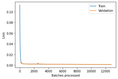
Finally, the training results are printed to assess the prediction on the test set by the trained model.
# the predicted values by the trained model is printed for the test set
fcn.show_results()| altitude_m | capacity_f | dayl__s_ | prcp__mm_d | srad__W_m_ | swe__kg_m_ | tmax__deg | tmin__deg | vp__Pa_ | wind_speed | prediction_results | |
|---|---|---|---|---|---|---|---|---|---|---|---|
| 0 | 1095 | 0.259311 | 58752.000000 | 0 | 403.200012 | 0 | 17.0 | 4.0 | 680 | 6.649275 | 0.261776 |
| 1 | 1095 | 0.299407 | 58752.000000 | 0 | 425.600006 | 0 | 19.5 | 5.5 | 720 | 6.135775 | 0.257786 |
| 2 | 1070 | 0.163723 | 40435.199219 | 0 | 361.600006 | 44 | 5.0 | -11.5 | 200 | 6.352946 | 0.109318 |
| 3 | 1095 | 0.015052 | 27993.599609 | 0 | 118.400002 | 4 | 5.0 | -7.5 | 360 | 9.014780 | 0.019792 |
| 4 | 1095 | 0.000002 | 27648.000000 | 1 | 105.599998 | 20 | -10.5 | -20.5 | 120 | 7.204670 | -0.003998 |
| 5 | 1055 | 0.074072 | 33868.800781 | 0 | 176.000000 | 0 | 11.0 | -1.5 | 560 | 6.275743 | 0.077243 |
In the table above, the values predicted by the model when applied to the test set, prediction_results, are similar to the actual values of the test set, capacity_f.
As such, the model metrics of the trained model can be now estimated using the model.score function, which returns the r-squared metric of the fitted model.
# the model.score method from the tabular learner returns r-square
r_Square_fcn_test = fcn.score()
print('r_Square_fcn_test: ', round(r_Square_fcn_test,5))r_Square_fcn_test: 0.84533
The high r-square value indicates that the model has been trained well
Solar Energy Generation Forecast & Validation
The trained model(FullyConnectedNetwork) will now be used to predict the daily lifetime solar energy generation for the solar plant installed at the Southland Leisure Centre, since its installation in 2015. The aim is to validate the trained model and measure its performance of solar output estimation using only weather variables from the Southland Leisure Center.
Accordingly, the model.predict method from arcgis.learn is used with the daily weather variables as input for the mentioned site, ranging from September 2015 to December 2019, to predict daily solar energy output in KWh for that same time period. The predictors are automatically chosen from the input feature layer of southland_layer by the trained model without mentioning them explicitly, since their names are exactly same as those used to train the model.
# predicting using the predict function
southland_solar_layer_predicted = fcn.predict(southland_solar_layer, output_layer_name='prediction_layer')C:\Users\sup10432\.conda\envs\upsupervisedEnvAug11\lib\site-packages\arcgis\features\geo\_io\fileops.py:743: UserWarning: Discarding nonzero nanoseconds in conversion out_name=fc_name)
# print the predicted layer
southland_solar_layer_predicted# Access & visualize the dataframe from the predicted layer
test_pred_layer = southland_solar_layer_predicted.layers[0]
test_pred_layer_sdf = test_pred_layer.query().sdf
test_pred_layer_sdf.head()| FID | fid_1 | field1 | id | solar_plan | altitude_m | latitude | longitude | wind_speed | dayl_s_ | ... | vp_pa_ | k_wh_fille | capacity_f | global_id | creation_d | creator | edit_date | editor | prediction | SHAPE | |
|---|---|---|---|---|---|---|---|---|---|---|---|---|---|---|---|---|---|---|---|---|---|
| 0 | 1 | 401 | 2016-07-05 | 164440 | Southland Leisure Centre | 1100 | 50.962485 | -114.108472 | 3.787571 | 58060.800781 | ... | 920 | 593.275 | 0.161567 | 3cbc6ed1-6504-4f41-8e4b-b95c62816070 | 2020-04-27 | arcgis_python | 2020-04-27 | arcgis_python | 0.202823 | {"x": -12702497.020502415, "y": 6614660.374377... |
| 1 | 2 | 402 | 2016-07-06 | 164440 | Southland Leisure Centre | 1100 | 50.962485 | -114.108472 | 3.302310 | 58060.800781 | ... | 920 | 575.397 | 0.156699 | d19858dc-1caa-4893-9e98-1540753eec4a | 2020-04-27 | arcgis_python | 2020-04-27 | arcgis_python | 0.190378 | {"x": -12702497.020502415, "y": 6614660.374377... |
| 2 | 3 | 403 | 2016-07-07 | 164440 | Southland Leisure Centre | 1100 | 50.962485 | -114.108472 | 3.923609 | 58060.800781 | ... | 880 | 886.423 | 0.241401 | 0ede54fa-3541-45be-9b64-5cdf259f69aa | 2020-04-27 | arcgis_python | 2020-04-27 | arcgis_python | 0.226812 | {"x": -12702497.020502415, "y": 6614660.374377... |
| 3 | 4 | 404 | 2016-07-08 | 164440 | Southland Leisure Centre | 1100 | 50.962485 | -114.108472 | 4.375310 | 57715.199219 | ... | 1000 | 976.136 | 0.265832 | c7259240-55a6-40fe-8700-844fafc12b8f | 2020-04-27 | arcgis_python | 2020-04-27 | arcgis_python | 0.218669 | {"x": -12702497.020502415, "y": 6614660.374377... |
| 4 | 5 | 405 | 2016-07-09 | 164440 | Southland Leisure Centre | 1100 | 50.962485 | -114.108472 | 2.816725 | 57715.199219 | ... | 1000 | 490.250 | 0.133510 | 6e59869a-e4e3-473a-b98f-a57ec6a5b480 | 2020-04-27 | arcgis_python | 2020-04-27 | arcgis_python | 0.179353 | {"x": -12702497.020502415, "y": 6614660.374377... |
5 rows × 25 columns
test_pred_layer_sdf.shape(1590, 25)
The table above returns the predicted values for the Southland photovoltaic power plant stored in the field called prediction_results, which holds the model estimated daily capacity factor of energy generation, whereas the actual capacity factor is in the field named capacity_f.
The capacity factor is a normalized value that will be rescaled back to the original unit of KWh by using the peak capacity of the Southland photovoltaic power plant of 153KWp.
# inverse scaling from capcacity factor to actual generation in KWh  - peak capcity of Southland Leisure Centre is 153KWp
test_pred_datetime = test_pred_layer_sdf[['field1','capacity_f','prediction']].copy()
test_pred_datetime = test_pred_datetime.rename(columns={'field1':'date'})
test_pred_datetime['date'] = pd.to_datetime(test_pred_datetime['date'])
test_pred_datetime = test_pred_datetime.set_index(test_pred_datetime['date'])
test_pred_datetime['Actual_generation(KWh)'] = test_pred_datetime['capacity_f']*24*153
test_pred_datetime['predicted_generation(KWh)'] = test_pred_datetime['prediction']*24*153
test_pred_datetime = test_pred_datetime.drop(['date','capacity_f','prediction'], axis=1).sort_index()
test_pred_datetime| Actual_generation(KWh) | predicted_generation(KWh) | |
|---|---|---|
| date | ||
| 2015-09-01 | 286.013 | 672.612955 |
| 2015-09-02 | 681.646 | 566.551533 |
| 2015-09-03 | 647.906 | 553.634092 |
| 2015-09-04 | 102.448 | 229.400620 |
| 2015-09-05 | 93.432 | 195.826120 |
| ... | ... | ... |
| 2019-12-27 | 1.349 | 37.905438 |
| 2019-12-28 | 1.965 | 12.047412 |
| 2019-12-29 | 1.616 | 69.387516 |
| 2019-12-30 | 7.440 | 114.383683 |
| 2019-12-31 | 8.323 | 69.632977 |
1590 rows × 2 columns
The table above shows the actual versus the model predicted daily solar energy generated for the Southland plant for the duration of late 2015 to the end of 2019. These values are now used to estimate the various model metrics to understand the prediction power of the model.
# estimate model metrics of r-square, rmse and mse for the actual and predicted values for daily energy generation
from sklearn.metrics import r2_score
r2_test = r2_score(test_pred_datetime['Actual_generation(KWh)'],test_pred_datetime['predicted_generation(KWh)'])
print('R-Square: ', round(r2_test, 2))
R-Square: 0.86
The comparison returns a high r-square of 0.86, showing a high similarity between the actual and predicted values.
# Comparison between the actual sum of the total energy generated to the total predicted values
actual = (test_pred_datetime['Actual_generation(KWh)'].sum()/4/1000).round(2)
predicted = (test_pred_datetime['predicted_generation(KWh)'].sum()/4/1000).round(2)
print('Actual annual Solar Energy Generated by Southland Solar Station: {} MWh'.format(actual))
print('Predicted annual Solar Energy Generated by Southland Solar Stations: {} MWh'.format(predicted))
Actual annual Solar Energy Generated by Southland Solar Station: 170.03 MWh Predicted annual Solar Energy Generated by Southland Solar Stations: 170.34 MWh
Summarizing the values, the actual average annual energy generated by the solar plant is 170.03 MWh which is close to the predicted annual average generated energy of 170.34 MWh, indicating a high level high precision.
Result Visualization
Finally, the actual and predicted values are plotted to visualize their distribution across the entire lifetime of the power plant.
plt.figure(figsize=(30,6))
plt.plot(test_pred_datetime['Actual_generation(KWh)'],  linewidth=1, label= 'Actual')
plt.plot(test_pred_datetime['predicted_generation(KWh)'], linewidth=1, label= 'Predicted')
plt.ylabel('Solar Energy in KWh', fontsize=14)
plt.legend(fontsize=14,loc='upper right')
plt.title('Actual Vs Predicted Solar Energy Generated by Southland Solar-FulyConnectedNetwork Model', fontsize=14)
plt.grid()
plt.show() 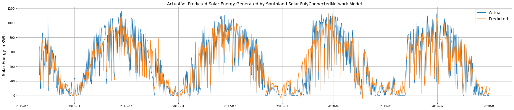
In the plot above, the blue line represents the actual generation values, and the orange line represents the predicted generation values. The two show a high degree of overlap, indicating that the model has a high predictive capacity.
MLModel
In the second method, a machine learning model is applied to model the same data using the MLModel framework from arcgis.learn. This framework can be used to import and apply any machine learning model from the scikit-learn library on the data returned by the prepare_tabulardata function from arcgis.learn.
# importing the libraries from arcgis.learn for data preprocessing for the Machine Learning Model
from sklearn.preprocessing import MinMaxScaler
Data Preprocessing
Like the data preparation process for the neural network, first a list is made consisting of the feature data that will be used for predicting daily solar energy generation. By default, it will receive continuous variables, whereas for categorical variables, the True value should be passed inside a tuple along with the variables. These variables are then transformed by the RobustScaler function from scikit-learn by passing it, along with the variable list, into the column transformer function as follows:
# scaling the feature data using MinMaxScaler(), the default is Normalizer from scikit learn
X = ['altitude_m', 'wind_speed', 'dayl__s_', 'prcp__mm_d','srad__W_m_','swe__kg_m_','tmax__deg','tmin__deg','vp__Pa_']
preprocessors =  [('altitude_m', 'wind_speed', 'dayl__s_', 'prcp__mm_d','srad__W_m_','swe__kg_m_','tmax__deg',
                   'tmin__deg','vp__Pa_', MinMaxScaler())]
Once the explanatory variables list is defined and the preprocessors are computed, they are now used as input for the prepare_tabulardata method in arcgis.learn. The method takes a feature layer or a spatial dataframe containing the dataset and returns a TabularDataObject that can be fed into the model.
The input parameters required for the tool are similar to the ones mentioned previously:
# importing the library from arcgis.learn for prepare data
from arcgis.learn import prepare_tabulardata
# precrocessing data using prepare data method for MLModel
data = prepare_tabulardata(calgary_no_southland_solar_layer,
'capacity_f',
explanatory_variables=X,
preprocessors=preprocessors)# check the data that is being trained
data.show_batch()| altitude_m | capacity_f | dayl__s_ | prcp__mm_d | srad__W_m_ | swe__kg_m_ | tmax__deg | tmin__deg | vp__Pa_ | wind_speed | |
|---|---|---|---|---|---|---|---|---|---|---|
| 146 | 1095 | 0.008051 | 38707.199219 | 0 | 329.600006 | 8 | 3.0 | -13.5 | 200 | 4.242083 |
| 170 | 1095 | 0.025921 | 33177.601562 | 3 | 70.400002 | 0 | 3.5 | -2.5 | 520 | 5.934033 |
| 391 | 1095 | 0.273637 | 57715.199219 | 0 | 515.200012 | 0 | 26.5 | 4.5 | 480 | 6.532143 |
| 522 | 1095 | 0.016343 | 32140.800781 | 0 | 147.199997 | 0 | -11.5 | -20.0 | 120 | 4.157886 |
| 825 | 1095 | 0.019354 | 29376.000000 | 0 | 102.400002 | 4 | 10.0 | 1.5 | 680 | 6.422836 |
| ... | ... | ... | ... | ... | ... | ... | ... | ... | ... | ... |
| 8390 | 1051 | 0.285307 | 56332.800781 | 0 | 460.799988 | 0 | 27.0 | 8.5 | 520 | 3.335872 |
| 8460 | 1051 | 0.233103 | 54604.800781 | 4 | 300.799988 | 0 | 26.5 | 10.0 | 1200 | 3.828789 |
| 8777 | 1051 | 0.285116 | 57369.601562 | 0 | 537.599976 | 0 | 27.5 | 5.5 | 320 | 4.703076 |
| 9035 | 1096 | 0.002692 | 27993.599609 | 0 | 134.399994 | 0 | -5.5 | -30.0 | 40 | 8.036874 |
| 9056 | 1096 | 0.122572 | 30412.800781 | 0 | 121.599998 | 0 | 4.5 | -6.0 | 400 | 7.787962 |
64 rows × 10 columns
Model Initialization
Once the data has been prepared by prepare_tabulardatamethod, it is ready to be passed to the selected machine learning model for training. Here, the GradientBoostingRegressor model from scikit-learn is used, which is passed into the MLModelfunction, along with its parameters, as follows:
# importing the MLModel framework from arcgis.learn and the model from scikit learn
from arcgis.learn import MLModel

# defining the model along with the parameters
model = MLModel(data, 'sklearn.ensemble.GradientBoostingRegressor', n_estimators=100, random_state=43)
Model Training
Finally, the model is now ready for training, and the model.fit method is used for fitting the machine learning model with its defined parameters mentioned in the previous step.
model.fit() The training results are printed to compute some model metrics and assess the quality of the trained model.
model.show_results()| altitude_m | capacity_f | dayl__s_ | prcp__mm_d | srad__W_m_ | swe__kg_m_ | tmax__deg | tmin__deg | vp__Pa_ | wind_speed | capacity_f_results | |
|---|---|---|---|---|---|---|---|---|---|---|---|
| 2564 | 1112 | 0.231209 | 58752.000000 | 0 | 432.000000 | 0 | 20.0 | 5.5 | 720 | 5.499134 | 0.222301 |
| 5576 | 1070 | 0.160846 | 58406.398438 | 3 | 208.000000 | 0 | 15.5 | 7.5 | 1040 | 3.904377 | 0.117711 |
| 7078 | 1090 | 0.167478 | 35596.800781 | 0 | 176.000000 | 0 | 6.0 | -3.5 | 480 | 7.295055 | 0.068521 |
| 8238 | 1051 | 0.000007 | 27648.000000 | 0 | 115.199997 | 8 | -6.5 | -18.5 | 160 | 7.262257 | 0.006838 |
| 9066 | 1096 | 0.097843 | 32140.800781 | 0 | 147.199997 | 0 | -10.5 | -20.5 | 120 | 4.157886 | 0.023777 |
In the table above, the last column, capacity_f_results, returns the values predicted by the model, which are similar to the actual values in the target variable column, capacity_f.
Subsequently, the model metrics of the trained model are now estimated using the model.score() function, which currently returns the r-squared of the model fit as follows:
# r-square is estimated using the inbuilt model.score() from the tabular learner
print('r_square_test_rf: ', round(model.score(), 5))
r_square_test_rf: 0.81248
The high R-squared value indicates that the model has been trained well.
Explaining Predictor Importance of Solar Energy Generation
Once the model has been fitted, it would be interesting to understand the explanability of the model, or the factors that are responsbile for predicting solar energy generation from the several varaible used in the model. The feature_importances method is used for the same as follows:
import seaborn as snsfeature_imp_RF = model.feature_importances_
rel_feature_imp = 100 * (feature_imp_RF / max(feature_imp_RF))
rel_feature_imp = pd.DataFrame({'features':list(X), 'rel_importance':rel_feature_imp })
rel_feature_imp = rel_feature_imp.sort_values('rel_importance', ascending=False)
plt.figure(figsize=[15,4])
plt.yticks(fontsize=10)
ax = sns.barplot(x="rel_importance", y="features", data=rel_feature_imp, palette="BrBG")
plt.xlabel("Relative Importance", fontsize=10)
plt.ylabel("Features", fontsize=10)
plt.show()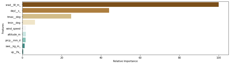
The above graph shows the feature importances returned by the featureimportances method of the trained Gradient Boosting regressor algorithm implemented via the MLModel framework. Here the most important predictor for forecasting solar energy generation at the site is shown to be the amount of solar radiation received by the site in watts per square meter (srad__W_m). This is followed by the length of day in seconds, maximum temperature and minimum temperature in the same order, which also matches the findings obtained from the correlation plot.
Solar Energy Generation Forecast & Validation
The trained GradientBoostingRegressor model, implemented via the MLModel, will now be used to predict the daily lifetime solar energy generation for the solar plant installed at the Southland Leisure Centre, since its installation in 2015. The aim is to compare and validate its performance to the performance of the FullyConnectedNetwork model developed in earlier in this lesson.
To reiterate, the model.predict method from arcgis.learn is used with the daily weather variables as input for the mentioned site, ranging from September 2015 to December 2019, to predict daily solar energy output in KWh for the same time period. The predictors are automatically chosen from the input feature layer of southland_layer by the trained model, without mentioning them explicitly, as their names are the same as those used for training the model.
southland_solar_layer_predicted_rf = model.predict(southland_solar_layer, output_layer_name='prediction_layer_rf')C:\Users\sup10432\.conda\envs\upsupervisedEnvAug11\lib\site-packages\arcgis\features\geo\_io\fileops.py:743: UserWarning: Discarding nonzero nanoseconds in conversion out_name=fc_name)
# print the predicted layer
southland_solar_layer_predicted_rf# Access & visualize the dataframe from the predicted layer
valid_pred_layer = southland_solar_layer_predicted_rf.layers[0]
valid_pred_layer_sdf = valid_pred_layer.query().sdf
valid_pred_layer_sdf.head()| FID | fid_1 | field1 | id | solar_plan | altitude_m | latitude | longitude | wind_speed | dayl_s_ | ... | vp_pa_ | k_wh_fille | capacity_f | global_id | creation_d | creator | edit_date | editor | prediction | SHAPE | |
|---|---|---|---|---|---|---|---|---|---|---|---|---|---|---|---|---|---|---|---|---|---|
| 0 | 1 | 1 | 2019-10-03 | 164440 | Southland Leisure Centre | 1100 | 50.962485 | -114.108472 | 5.332239 | 40089.601562 | ... | 480 | 309.644 | 0.084326 | e9b0f671-d6ba-4560-b912-d635a0a129f8 | 2020-04-27 | arcgis_python | 2020-04-27 | arcgis_python | 0.124855 | {"x": -12702497.020502415, "y": 6614660.374377... |
| 1 | 2 | 2 | 2019-10-04 | 164440 | Southland Leisure Centre | 1100 | 50.962485 | -114.108472 | 6.304829 | 40089.601562 | ... | 560 | 679.785 | 0.185127 | 7bde5210-a8c2-4731-9c23-e5f77c1ebc56 | 2020-04-27 | arcgis_python | 2020-04-27 | arcgis_python | 0.148331 | {"x": -12702497.020502415, "y": 6614660.374377... |
| 2 | 3 | 3 | 2019-10-05 | 164440 | Southland Leisure Centre | 1100 | 50.962485 | -114.108472 | 7.631040 | 39744.000000 | ... | 720 | 581.859 | 0.158458 | acfd49e7-3973-49b6-9077-f12ab0c44af1 | 2020-04-27 | arcgis_python | 2020-04-27 | arcgis_python | 0.134697 | {"x": -12702497.020502415, "y": 6614660.374377... |
| 3 | 4 | 4 | 2019-10-06 | 164440 | Southland Leisure Centre | 1100 | 50.962485 | -114.108472 | 8.590591 | 39398.398438 | ... | 720 | 718.478 | 0.195664 | 27d3b8bb-aabe-4e70-acc3-579882d43b01 | 2020-04-27 | arcgis_python | 2020-04-27 | arcgis_python | 0.143388 | {"x": -12702497.020502415, "y": 6614660.374377... |
| 4 | 5 | 5 | 2019-10-07 | 164440 | Southland Leisure Centre | 1100 | 50.962485 | -114.108472 | 10.636899 | 39398.398438 | ... | 640 | 406.956 | 0.110827 | 9885c59a-d0b2-4956-ad97-4c8ec6483aab | 2020-04-27 | arcgis_python | 2020-04-27 | arcgis_python | 0.113309 | {"x": -12702497.020502415, "y": 6614660.374377... |
5 rows × 25 columns
The table above returns the MLModel predicted values for the Southland plant stored in the field prediction, while the actual capacity factor is stored in the field named capacity_f.
The capacity factor is a normalized value that will be rescaled back to the original unit of KWh by using the peak capacity of the Southland photovoltaic power plant of 153KWp.
# inverse scaling from capcacity factor to actual generation in KWh  - peak capcity of Southland Leisure Centre is 153KWp
valid_pred_datetime = valid_pred_layer_sdf[['field1','capacity_f','prediction']].copy()
valid_pred_datetime = valid_pred_datetime.rename(columns={'field1':'date'})
valid_pred_datetime['date'] = pd.to_datetime(valid_pred_datetime['date'])
valid_pred_datetime = valid_pred_datetime.set_index(valid_pred_datetime['date'])
valid_pred_datetime['Actual_generation(KWh)'] = valid_pred_datetime['capacity_f']*24*153
valid_pred_datetime['predicted_generation(KWh)'] = valid_pred_datetime['prediction']*24*153
valid_pred_datetime = valid_pred_datetime.drop(['date','capacity_f','prediction'], axis=1)
valid_pred_datetime = valid_pred_datetime.sort_index()
valid_pred_datetime.head()| Actual_generation(KWh) | predicted_generation(KWh) | |
|---|---|---|
| date | ||
| 2015-09-01 | 286.013 | 718.458356 |
| 2015-09-02 | 681.646 | 679.957975 |
| 2015-09-03 | 647.906 | 548.296796 |
| 2015-09-04 | 102.448 | 195.091296 |
| 2015-09-05 | 93.432 | 132.086403 |
The table above shows the actual versus the MLModel predicted daily solar energy generated for the Southland plant for the duration of late 2015 to the end of 2019. These values are now used to estimate the various model metrics to understand the prediction power of the MLModel.
# estimate model metrics of r-square, rmse and mse for the actual and predicted values for daily energy generation
from sklearn.metrics import r2_score
r2_test = r2_score(valid_pred_datetime['Actual_generation(KWh)'],valid_pred_datetime['predicted_generation(KWh)'])
print('R-Square: ', round(r2_test, 2))
R-Square: 0.84
The comparison returns a high R-squared of 0.84, indicating a high similarity between the actual and predicted values.
# Comparison between the actual sum of the total energy generated to the total predicted values by the MLModel
actual = (valid_pred_datetime['Actual_generation(KWh)'].sum()/4/1000).round(2)
predicted = (valid_pred_datetime['predicted_generation(KWh)'].sum()/4/1000).round(2)
print('Actual annual Solar Energy Generated by Southland Solar Station: {} MWh'.format(actual))
print('Predicted annual Solar Energy Generated by Southland Solar Stations: {} MWh'.format(predicted))
Actual annual Solar Energy Generated by Southland Solar Station: 170.03 MWh Predicted annual Solar Energy Generated by Southland Solar Stations: 171.48 MWh
Summarizing the values, the actual average annual energy generated by the solar plant is 170.03 MWh, which is close to the predicted annual average generated energy of 171.48 MWh. This indicates a high level of precision.
Result Visualization
Finally, the actual and predicted values are plotted to visualize their distribution across the entire lifetime of the power plant.
plt.figure(figsize=(30,6))
plt.plot(valid_pred_datetime['Actual_generation(KWh)'],  linewidth=1, label= 'Actual')
plt.plot(valid_pred_datetime['predicted_generation(KWh)'], linewidth=1, label= 'Predicted')
plt.ylabel('Solar Energy in KWh', fontsize=14)
plt.legend(fontsize=14,loc='upper right')
plt.title('Actual Vs Predicted Solar Energy Generated by Southland Solar-FulyConnectedNetwork Model', fontsize=14)
plt.grid()
plt.show() 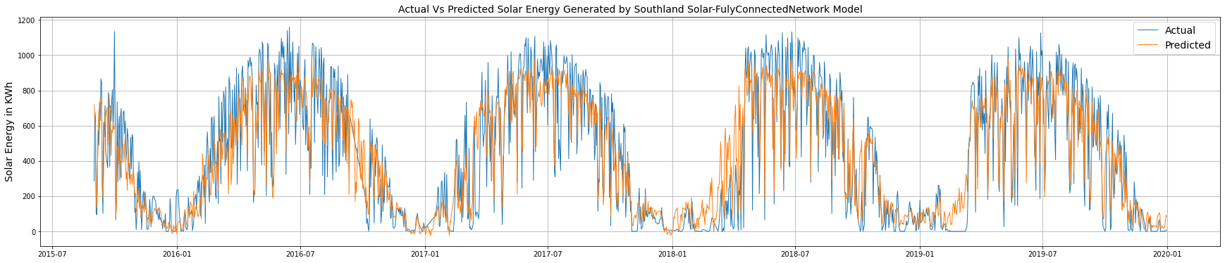
Conclusion
The goal of this project was to create a model that could predict the daily solar energy efficiency, thereby estimate the actual output of a photovoltaic solar energy plant at a location using the daily weather variables of the site as inputs. In the process it demonstrated the newly implemented artificial neural network, called FullyConnectedNetwork, and machine learning models, called MLModel, available in the arcgis.learn module in ArcGIS API for Python.
Accordingly, data from 10 solar energy installation sites in the City of Calgary in Canada were used to train two different models — the first being the FullyConnectedNetwork model and second being the MLModel framework from the arcgis.learn module. These were eventually used to predict the daily solar output of a different solar plant in Calgary, which was withheld from the training set. The steps for implementing these models are elaborated in the notebook, and include the steps of data preprocessing, model training, and final inferencing.
Comparison of the result shows that both models successfully predicted the solar energy output of the test solar plant with predicted values of 170.34 MWh and 171.48 MWh by the FullyConnectedNetwork and the MLModel algorithm respectively, compared to the actual value of average annual solar generation of 170.03 MWh for the station.
Finally, to expand on this model further in the furture, it would be interesting to apply this model to other solar generation plants located across different geographies and to record its performance to understand the generalizability of the model.
Summary of methods used
| Method | Description | Examples |
|---|---|---|
| prepare_tabulardata | prepare data including imputation, normalization and train-test split | prepare data ready for fitting a MLModel or FullyConnectedNetwork model |
| FullyConnectedNetwork() | set a fully connected neural network to a data | initialize a FullyConnectedNetwork model with prepared data |
| model.lr_find() | find an optimal learning rate | finalize a good learning rate for training the FullyConnectedNetwork model |
| MLModel() | select the ML algorithm to be used for fitting | any supervised or unsupervised regression and classification model from scikit learn can be used |
| model.fit() | train a model with epochs & learning rate as input | training the FullyConnectedNetwork model with sutiable input |
| model.score() | find the model metric of R-squared of the trained model | returns R-squared value after training the MLModel and FullyConnectedNetwork model |
| model.predict() | predict on a test set | predict values using the trained models on test input |
Data resources
| Dataset | Source | Link |
|---|---|---|
| Calgary solar energy | Calgary daily solar energy generation | https://data.calgary.ca/Environment/Solar-Energy-Production/ytdn-2qsp |
| Calgary Photovoltaic Sites | Location of Calgary Solar sites in Lat & Lon | https://data.calgary.ca/dataset/City-of-Calgary-Solar-Photovoltaic-Sites/vrdj-ycb5 |
| Calgary Daily weather data | MODIS - Daily Surface Weather Data on a 1-km Grid for North America, Version 3 | https://daac.ornl.gov/DAYMET/guides/Daymet_V3_CFMosaics.html |