Temperature forecast using time series data

Introduction

Weather forecasting has been a significant area for application of advanced deep learning and machine learning methodologies over traditional methods to improve weather prediction. These new methods are appropriate for processing large chunks of data where massive quantity of historic weather datasets could be utilized for forecasting. This sample showcases two autoregressive methods: one using a deep learning and another using a machine learning framework to predict temperature of England.

Historic temperature data from various weather stations across England is collected from here. The data consists of daily temperature measurements ranging from February 2005 till September 2019 which are auto regressed to predict daily temperature for each of the identified stations for October 2019. The forecasted temperature obtained for the stations is then spatially interpolated using ArcGIS spatial interpolation tool to produce a temperature prediction surface for the entire country. Here is a schematic flow chart of the operation:

Prerequisites

Some required libraries for this sample are NumPy for processing arrays, pandas for operating with DataFrame, ArcGIS for geoprocessing, scikit-learn=0.22.1 for machine learning, tensorflow=2.0.0 and keras=2.2.4 for deep learning.

Necessary Imports

%matplotlib inline
import matplotlib.pyplot as plt

import numpy as np
import pandas as pd
import math
from datetime import datetime as dt
from IPython.display import Image, HTML

from sklearn.svm import SVR
from sklearn.preprocessing import MinMaxScaler
from sklearn.metrics import mean_squared_error, r2_score

from tensorflow.keras.models import Sequential
from tensorflow.keras.layers import LSTM, Dense, Activation, Dropout
from tensorflow.keras.optimizers import Adam
import tensorflow.keras.backend as K

from arcgis.gis import GIS
from arcgis.features.analysis import interpolate_points

Connect to your GIS

gis = GIS(profile='your_online_profile')

Obtain and Visualize Data for Analysis

The primary data used for this sample is as follows:

Data 1— England Boundary

First the boundary of England shapefile is accessed. This will be used to interpolate temperature within this particular area.

# Access England Boundary
england_border = gis.content.get('0856d38fea9149a48227cdc2f1e4f4f6')
england_border

england1

Feature Layer Collection by api_data_owner
Last Modified: November 22, 2024
0 comments, 96 views

# Get the feature layer
england_boundary_layer = england_border.layers[0]

# Plot England boundary
england_map = gis.map('England')
england_map.content.add(england_boundary_layer)
england_map.basemap.basemap = 'topo-vector'
england_map

england_map.zoom = 6

Data 2 — England Weather Stations

There are several weather stations in England that record a variety of weather data. Here 29 weather stations are strategically selected such that they are well distributed across England and can be used to forecast temperature which will cover the entire country. These include stations located at prominent English cities such as London, Birmingham, Cardiff, Exeter, Nottingham, Plymouth and others, as shown in the map below.

# Access England Weather Stations
england_weather_stations = gis.content.get('fd3ecbd95b7148b8a7cbcc866cedd514')
england_weather_stations

england_weather_stations1

Feature Layer Collection by api_data_owner
Last Modified: December 20, 2019
0 comments, 48 views

england_weather_stations_layer = england_weather_stations.layers[0]

# England weather stations
england_weather_stations_map = gis.map('England')
england_weather_stations_map.basemap.basemap = 'topo-vector'
england_weather_stations_map.content.add(england_weather_stations_layer)
england_weather_stations_map

england_weather_stations_map.zoom = 6

The locations of the weather stations are mapped here which are uniformly distributed throughout England. This is necessary to create a well interpolated prediction surface. The more the number of weather stations, more precise would be the interpolated result.

# Access spatial dataframe
england_weather_stations_layer_sdf = pd.DataFrame.spatial.from_layer(england_weather_stations_layer)
england_weather_stations_layer_sdf.head()

	FID	Station	Y	X	SHAPE
0	1	Albemarle	55.016667	-1.866667	{"x": -207796.38285121127, "y": 7365101.445978...
1	2	Begwary	52.216667	-0.483333	{"x": -53804.420512971476, "y": 6839396.777444...
2	3	Birmingham_airport	52.45	-1.733333	{"x": -192953.78400456344, "y": 6881903.804921...
3	4	Blackpool_airport	53.766667	-3.033333	{"x": -337669.1220358203, "y": 7126089.0211904...
4	5	Boulmer_airport	55.4203	-1.5997	{"x": -178077.78942199165, "y": 7443868.808735...

The table above shows the latitude (Y) and longitude (X) values of the 29 weather station used in this study.

Data 3 — Historic Temperature

Daily Mean temperature in degree Celsius ranging from February, 2005 till September,2019 is accessed from the above mentioned weather stations. One issue with timeseries datasets that needed to be addressed was missing data. Thus, weather stations with the least amount of missing data were selected for the study.

# Access historic temperature data of England
table = gis.content.get('d15eba5e9fe54a968e272c32d8e58e1f')

temp_history = table.tables[0]

# Visualize as pandas dataframe
all_station_temp_history = temp_history.query().sdf

all_station_temp_history.tail()

	Date	Albemarle	Begwary	Birmingham_airport	Blackpool_airport	Boulmer_airport	Bournemouth_airport	BrizeNorton_airport	Cardiff_airport	Carlisle	...	Nottingham	Plymouth_weatherstation	Rostherne	Scampton_airport	Shawbury_airport	Southend_on_Sea_AWS	Stansted_airport	Wittering_airport	Yeovilton_airport	ObjectId
5350	26-09-2019	13.79	16.15	15.62	15.24	<NA>	16.99	15.95	15.77	14.1	...	14.46	15.96	14.9	15.21	14.65	17.16	16.27	15.85	16.64	5351
5351	27-09-2019	10.9	13.72	13.28	13.72	<NA>	15.08	14.05	14.88	12.25	...	12.79	14.6	12.77	13.05	13.37	15.76	14.21	13.22	14.95	5352
5352	28-09-2019	11.26	14.11	13.9	14.12	<NA>	15.95	14.31	15.33	12.37	...	13.46	15.03	13.67	13.36	13.91	15.68	14.19	14.1	15.37	5353
5353	29-09-2019	10.68	15.25	14.79	12.68	<NA>	15.88	15.38	14.98	11.8	...	13.66	15.19	13.19	13.49	14.14	16.18	15.31	14.74	15.65	5354
5354	30-09-2019	10.1	12.91	12.73	13.6	<NA>	14.22	13.14	14.27	11.08	...	12.11	14.78	12.12	12.08	12.02	14.31	13.5	12.56	13.7	5355

5 rows × 31 columns

all_station_temp_history.shape

(5355, 31)

england_temp = all_station_temp_history[all_station_temp_history.columns[0:30]]

england_temp.tail()

	Date	Albemarle	Begwary	Birmingham_airport	Blackpool_airport	Boulmer_airport	Bournemouth_airport	BrizeNorton_airport	Cardiff_airport	Carlisle	...	Norwich_airport	Nottingham	Plymouth_weatherstation	Rostherne	Scampton_airport	Shawbury_airport	Southend_on_Sea_AWS	Stansted_airport	Wittering_airport	Yeovilton_airport
5350	26-09-2019	13.79	16.15	15.62	15.24	<NA>	16.99	15.95	15.77	14.1	...	16.6	14.46	15.96	14.9	15.21	14.65	17.16	16.27	15.85	16.64
5351	27-09-2019	10.9	13.72	13.28	13.72	<NA>	15.08	14.05	14.88	12.25	...	13.89	12.79	14.6	12.77	13.05	13.37	15.76	14.21	13.22	14.95
5352	28-09-2019	11.26	14.11	13.9	14.12	<NA>	15.95	14.31	15.33	12.37	...	14.42	13.46	15.03	13.67	13.36	13.91	15.68	14.19	14.1	15.37
5353	29-09-2019	10.68	15.25	14.79	12.68	<NA>	15.88	15.38	14.98	11.8	...	15.46	13.66	15.19	13.19	13.49	14.14	16.18	15.31	14.74	15.65
5354	30-09-2019	10.1	12.91	12.73	13.6	<NA>	14.22	13.14	14.27	11.08	...	13.87	12.11	14.78	12.12	12.08	12.02	14.31	13.5	12.56	13.7

5 rows × 30 columns

The table above shows the historic temperature data in degree Celsius of all the weather stations starting from 2005 to September 2019. The first column is the Date field which is the day of the recorded temperature and rest of the columns are weather stations.

Convert to Timeseries format

This temperature dataset is now transformed into a timeseries data format where the Date column is set as the index of the dataset.

# Change to datetime format
england_temp_new = england_temp.copy() 
england_temp_new[england_temp_new.columns[0]] = pd.to_datetime(england_temp_new[england_temp_new.columns[0]], format='%d-%m-%Y')
england_temp_new = england_temp_new.set_index(england_temp_new.columns[0])
england_temp_new = england_temp_new.sort_index()
all_station_temp = england_temp_new.astype('float')
all_station_temp.tail()

	Albemarle	Begwary	Birmingham_airport	Blackpool_airport	Boulmer_airport	Bournemouth_airport	BrizeNorton_airport	Cardiff_airport	Carlisle	Crosby	...	Norwich_airport	Nottingham	Plymouth_weatherstation	Rostherne	Scampton_airport	Shawbury_airport	Southend_on_Sea_AWS	Stansted_airport	Wittering_airport	Yeovilton_airport
Date
2019-09-26	13.79	16.15	15.62	15.24	NaN	16.99	15.95	15.77	14.10	15.45	...	16.60	14.46	15.96	14.90	15.21	14.65	17.16	16.27	15.85	16.64
2019-09-27	10.90	13.72	13.28	13.72	NaN	15.08	14.05	14.88	12.25	13.96	...	13.89	12.79	14.60	12.77	13.05	13.37	15.76	14.21	13.22	14.95
2019-09-28	11.26	14.11	13.90	14.12	NaN	15.95	14.31	15.33	12.37	14.40	...	14.42	13.46	15.03	13.67	13.36	13.91	15.68	14.19	14.10	15.37
2019-09-29	10.68	15.25	14.79	12.68	NaN	15.88	15.38	14.98	11.80	13.29	...	15.46	13.66	15.19	13.19	13.49	14.14	16.18	15.31	14.74	15.65
2019-09-30	10.10	12.91	12.73	13.60	NaN	14.22	13.14	14.27	11.08	13.82	...	13.87	12.11	14.78	12.12	12.08	12.02	14.31	13.50	12.56	13.70

5 rows × 29 columns

Model Building

Once the dataset is transformed into a timeseries dataset, it is ready to be used for modelling. In this sample two types of methodology are used for modelling:

1) LSTM - First a deep learning framework of LSTM is used which is appropriate for handling time series data.

2) Support Vector Machine - In the second option the machine learning algorithm of Support Vector Regression(SVR) is used to compare the performance between the two methods in terms of accuracy and computation time.

LSTM

LSTM (Long short-term memory) first proposed by Hochreiter & Schmidhuber, is a type of Recurrent Neural Network(RNN). RNN could be defined as a special kind of neural network which can retain information from past inputs which is not possible for traditional neural networks. This makes it suitable for forecasting timeseries data wherein prediction is done based on past data. LSTM is built of units, each consisting of four neural networks, which are used to update its cell state using information from new inputs and past outputs.

A function is created here which encapsulates the steps for processing and predicting from the timeseries data.

First an empty datetime DataFrame is created for the number of days the temperature is to be forecasted, where future predicted values will be stored.

# create future forecast dates
def create_dates(start,days):
    v = pd.date_range(start=start, periods=days+1, freq='D', inclusive='right')
    seven_day_forecast = pd.DataFrame(index=v) 
    return seven_day_forecast

This next method accesses the station name from the input data and the related values for that station.

# get values, station name and drop null values
def get_value_name(all_station_temp,i):
    station_value = all_station_temp[[all_station_temp.columns[i]]].dropna()
    station_name = all_station_temp.columns[i]
    return station_value, station_name

Sequence of a timeseries is very important, hence while splitting the values into train and test set, the order is to be retained. This method takes the above accessed values and divides it into user input ratio before and after a certain date.

# train-test split for a user input ratio
def train_test_split(value, name, ratio):
    nrow = len(value)
    print(name+' total samples: ',nrow)
    split_row = int((nrow)*ratio)
    print('Training samples: ',split_row)
    print('Testing samples: ',nrow-split_row)
    train = value.iloc[:split_row]
    test = value.iloc[split_row:]
    return train, test, split_row

Data scaling is essential before feeding it to a LSTM, which helps it train better compared to raw unscaled data. This method scales the train and test data using a minmax scaler from sci-kit learn.

# data transformation
def data_transformation(train_tract1,test_tract1):
    scaler = MinMaxScaler()
    train_tract1_scaled = scaler.fit_transform(train_tract1)
    test_tract1_scaled = scaler.fit_transform(test_tract1)          
    train_tract1_scaled_df = pd.DataFrame(train_tract1_scaled, index = train_tract1.index, columns=[train_tract1.columns[0]])
    test_tract1_scaled_df = pd.DataFrame(test_tract1_scaled,
                                         index = test_tract1.index, columns=[test_tract1.columns[0]])
    return train_tract1_scaled_df, test_tract1_scaled_df, scaler

Finally one more transformation of feature engineering is required, which is to create new features using lagged values of the time series data itself. Here the number of lag terms could be specified and the function would create lag number of new features using the lagged terms.

# feature builder - This section creates feature set with lag number of predictors--Creating features using lagged data
def timeseries_feature_builder(df, lag):
    df_copy = df.copy()
    for i in range(1,lag):
        df_copy['lag'+str(i)] = df.shift(i) 
    return df_copy
    df_copy = df.copy()

Null values resulting from the above feature creation are dropped followed by converting the train and test values to arrays, which is the input data type for LSTM.

# preprocessing -- drop null values and make arrays 
def make_arrays(train_tract1,test_tract1):
    X_train_tract1_array = train_tract1.dropna().drop(train_tract1.columns[0], axis=1).values
    y_train_tract1_array = train_tract1.dropna()[train_tract1.columns[0]].values
    X_test_tract1_array = test_tract1.dropna().drop(test_tract1.columns[0], axis=1).values
    y_test_tract1_array = test_tract1.dropna()[test_tract1.columns[0]].values    
    return X_train_tract1_array, y_train_tract1_array, X_test_tract1_array, y_test_tract1_array

LSTM model with three hidden layer is created each having a user input number of LSTM memory units, with a dropout rate of 20% for each layer, and a final output dense layer predicting a single value.

# Define LSTM model
def lstm_model(units, trainX, testX, y_train_tract1_array, y_test_tract1_array):
    model = Sequential()
    model.add(LSTM(units,return_sequences=True, input_shape=(trainX.shape[1],trainX.shape[2]),kernel_initializer='lecun_uniform'))
    model.add(Dropout(0.2))    
    model.add(LSTM(units, return_sequences=True))
    model.add(Dropout(0.2))    
    model.add(LSTM(units))
    model.add(Dropout(0.2))
    model.add(Dense(1))        
    model.compile(optimizer=Adam(learning_rate=0.001), loss='mean_squared_error')
    
    model.fit(trainX, y_train_tract1_array, batch_size=120, epochs=100, validation_data=(testX, y_test_tract1_array), verbose=0)
    return model

In the validation method, the fitted model is used here to predict on the test set and the results are added to a column called Forecast for visualization. The accuracy of the predicted result is measured by r-square method, to check its similarity with the actual temperature readings, which is intuitive to interpret.

# validation result 
def valid_result(model, testX, y_test_tract1_array, scaler, station_value, split_row, lag):    
    testPredict = model.predict(testX)
    rSquare_test = r2_score(y_test_tract1_array, testPredict)
    print('Test R-squared is: %f'%rSquare_test)    
    testPredict = scaler.inverse_transform(testPredict)        
    new_test_tract1 = station_value.iloc[split_row:]       
    test_tract1_pred = new_test_tract1.iloc[lag:].copy()
    test_tract1_pred['Forecast'] = testPredict
    return test_tract1_pred

Once the results are validated, the model is used to forecast temperature for the next 31 days or the month of October, 2019 by a walk forward of each day. Here the past lag number of days are used to predict the temperature for October 1st. This predicted value is then included as a predictor for forecasting the next days value, and input into the fitted model along with past days temperatures, and so on till all the days are predicted. This is repeated for each weather station.

# multi step future forecast for next days number of days. 
def forecast(model, testX, test_tract1, lag, scaler, days):
    seven_days = []
    new0 = testX[-1]        
    last = test_tract1.iloc[-1]
    new_predict = last[0]        
    new_array = np.insert(new0, 0, new_predict)        
    new_array = np.delete(new_array, -1)
    new_array_reshape = np.reshape(new_array, (-1,1,lag))       
    new_predict = model.predict(new_array_reshape)
    temp_predict = scaler.inverse_transform(new_predict) 
    seven_days.append(temp_predict[0][0].round(2))
    
    for i in range(1,days):
        new_array = np.insert(new_array, 0, new_predict)             
        new_array = np.delete(new_array, -1)
        new_array_reshape = np.reshape(new_array, (-1,1,lag))            
        new_predict = model.predict(new_array_reshape)
        temp_predict = scaler.inverse_transform(new_predict) 
        seven_days.append(temp_predict[0][0].round(2))
    return seven_days

Finally the main function is created which calls the above modules for predicting the monthly forecast. This consists of first accessing time series data for each station, processing them into appropriate input format and fitting a LSTM model on 90% of the data as training set. This is followed by validating the trained model on the rest 10% of the data and final forecasting for the next 31 days using the trained model, which is then repeated for all the 29 station.

def england_temp_lstm(all_station_temp, lag, days):    
    
    seven_day_forecast_lstm = create_dates('2019-09-30',days) 
    
    for i in range(len(all_station_temp.columns)):
        
        # preprocessing
        station_value, station_name = get_value_name(all_station_temp,i)        
        train_tract1, test_tract1, split_row = train_test_split(station_value, station_name, 0.90)        
        train_tract1_scaled_df, test_tract1_scaled_df, scaler = data_transformation(train_tract1,test_tract1) 
        train_tract1 = timeseries_feature_builder(train_tract1_scaled_df, lag+1) 
        test_tract1 = timeseries_feature_builder(test_tract1_scaled_df, lag+1)               
        X_train_tract1_array, y_train_tract1_array, X_test_tract1_array, y_test_tract1_array = make_arrays(train_tract1, 
                                                                                                           test_tract1)        
        trainX = np.reshape(X_train_tract1_array, (X_train_tract1_array.shape[0],1,X_train_tract1_array.shape[1]))
        testX = np.reshape(X_test_tract1_array, (X_test_tract1_array.shape[0],1,X_test_tract1_array.shape[1]))                
        
        # LSTM modelling & forecast
        model = lstm_model(30, trainX, testX, y_train_tract1_array, y_test_tract1_array)             
        test_tract1_pred = valid_result(model, testX, y_test_tract1_array, scaler, station_value, split_row, lag)        
        seven_days = forecast(model, testX, test_tract1, lag, scaler, days)       
        seven_day_forecast_lstm[station_name] = np.array(seven_days)       
        
        # plot result
        plt.figure(figsize=(20,5))
        plt.plot(test_tract1_pred)        
        plt.plot(seven_day_forecast_lstm[station_name], color='red', label='forecast')         
        plt.ylabel('Temperature(°C)')
        plt.legend(loc='upper right')
        plt.title(station_name + '- October 2019 Temperature Forecast')
        plt.show()        
        
    return(seven_day_forecast_lstm)

Once the main function is ready it is called on the weather station dataset consisting of past temperature data from the selected weather stations. It is given three input: the data table, number of past day's data to be used for forecasting and the number of days for which the temperature is to be predicted.

%%time
# Fitting and forecast using LSTM  -- output of train loss and valid loss is turned off
lstm_prediction = england_temp_lstm(all_station_temp,120,31)

Albemarle total samples:  3648
Training samples:  3283
Testing samples:  365
8/8 [==============================] - 1s 2ms/step
Test R-squared is: 0.858284
1/1 [==============================] - 0s 24ms/step
1/1 [==============================] - 0s 24ms/step
1/1 [==============================] - 0s 24ms/step
1/1 [==============================] - 0s 22ms/step
1/1 [==============================] - 0s 24ms/step
1/1 [==============================] - 0s 22ms/step
1/1 [==============================] - 0s 22ms/step
1/1 [==============================] - 0s 26ms/step
1/1 [==============================] - 0s 23ms/step
1/1 [==============================] - 0s 23ms/step
1/1 [==============================] - 0s 23ms/step
1/1 [==============================] - 0s 23ms/step
1/1 [==============================] - 0s 23ms/step
1/1 [==============================] - 0s 23ms/step
1/1 [==============================] - 0s 22ms/step
1/1 [==============================] - 0s 25ms/step
1/1 [==============================] - 0s 25ms/step
1/1 [==============================] - 0s 26ms/step
1/1 [==============================] - 0s 25ms/step
1/1 [==============================] - 0s 22ms/step
1/1 [==============================] - 0s 23ms/step
1/1 [==============================] - 0s 24ms/step
1/1 [==============================] - 0s 24ms/step
1/1 [==============================] - 0s 25ms/step
1/1 [==============================] - 0s 24ms/step
1/1 [==============================] - 0s 24ms/step
1/1 [==============================] - 0s 25ms/step
1/1 [==============================] - 0s 24ms/step
1/1 [==============================] - 0s 22ms/step
1/1 [==============================] - 0s 24ms/step
1/1 [==============================] - 0s 23ms/step

Begwary total samples:  3648
Training samples:  3283
Testing samples:  365
8/8 [==============================] - 1s 2ms/step
Test R-squared is: 0.848154
1/1 [==============================] - 0s 24ms/step
1/1 [==============================] - 0s 24ms/step
1/1 [==============================] - 0s 25ms/step
1/1 [==============================] - 0s 23ms/step
1/1 [==============================] - 0s 23ms/step
1/1 [==============================] - 0s 24ms/step
1/1 [==============================] - 0s 25ms/step
1/1 [==============================] - 0s 24ms/step
1/1 [==============================] - 0s 26ms/step
1/1 [==============================] - 0s 25ms/step
1/1 [==============================] - 0s 26ms/step
1/1 [==============================] - 0s 24ms/step
1/1 [==============================] - 0s 23ms/step
1/1 [==============================] - 0s 25ms/step
1/1 [==============================] - 0s 25ms/step
1/1 [==============================] - 0s 24ms/step
1/1 [==============================] - 0s 25ms/step
1/1 [==============================] - 0s 24ms/step
1/1 [==============================] - 0s 25ms/step
1/1 [==============================] - 0s 25ms/step
1/1 [==============================] - 0s 24ms/step
1/1 [==============================] - 0s 25ms/step
1/1 [==============================] - 0s 26ms/step
1/1 [==============================] - 0s 25ms/step
1/1 [==============================] - 0s 25ms/step
1/1 [==============================] - 0s 23ms/step
1/1 [==============================] - 0s 23ms/step
1/1 [==============================] - 0s 26ms/step
1/1 [==============================] - 0s 26ms/step
1/1 [==============================] - 0s 23ms/step
1/1 [==============================] - 0s 24ms/step

Birmingham_airport total samples:  2556
Training samples:  2300
Testing samples:  256
5/5 [==============================] - 1s 1ms/step
Test R-squared is: 0.528638
1/1 [==============================] - 0s 22ms/step
1/1 [==============================] - 0s 23ms/step
1/1 [==============================] - 0s 24ms/step
1/1 [==============================] - 0s 24ms/step
1/1 [==============================] - 0s 24ms/step
1/1 [==============================] - 0s 23ms/step
1/1 [==============================] - 0s 23ms/step
1/1 [==============================] - 0s 23ms/step
1/1 [==============================] - 0s 23ms/step
1/1 [==============================] - 0s 24ms/step
1/1 [==============================] - 0s 24ms/step
1/1 [==============================] - 0s 26ms/step
1/1 [==============================] - 0s 26ms/step
1/1 [==============================] - 0s 25ms/step
1/1 [==============================] - 0s 25ms/step
1/1 [==============================] - 0s 26ms/step
1/1 [==============================] - 0s 25ms/step
1/1 [==============================] - 0s 24ms/step
1/1 [==============================] - 0s 24ms/step
1/1 [==============================] - 0s 25ms/step
1/1 [==============================] - 0s 23ms/step
1/1 [==============================] - 0s 24ms/step
1/1 [==============================] - 0s 23ms/step
1/1 [==============================] - 0s 23ms/step
1/1 [==============================] - 0s 23ms/step
1/1 [==============================] - 0s 25ms/step
1/1 [==============================] - 0s 26ms/step
1/1 [==============================] - 0s 25ms/step
1/1 [==============================] - 0s 25ms/step
1/1 [==============================] - 0s 24ms/step
1/1 [==============================] - 0s 23ms/step

Blackpool_airport total samples:  3501
Training samples:  3150
Testing samples:  351
8/8 [==============================] - 1s 1ms/step
Test R-squared is: 0.878246
1/1 [==============================] - 0s 23ms/step
1/1 [==============================] - 0s 24ms/step
1/1 [==============================] - 0s 24ms/step
1/1 [==============================] - 0s 25ms/step
1/1 [==============================] - 0s 25ms/step
1/1 [==============================] - 0s 25ms/step
1/1 [==============================] - 0s 22ms/step
1/1 [==============================] - 0s 22ms/step
1/1 [==============================] - 0s 22ms/step
1/1 [==============================] - 0s 21ms/step
1/1 [==============================] - 0s 22ms/step
1/1 [==============================] - 0s 23ms/step
1/1 [==============================] - 0s 23ms/step
1/1 [==============================] - 0s 21ms/step
1/1 [==============================] - 0s 24ms/step
1/1 [==============================] - 0s 23ms/step
1/1 [==============================] - 0s 22ms/step
1/1 [==============================] - 0s 24ms/step
1/1 [==============================] - 0s 23ms/step
1/1 [==============================] - 0s 21ms/step
1/1 [==============================] - 0s 25ms/step
1/1 [==============================] - 0s 24ms/step
1/1 [==============================] - 0s 22ms/step
1/1 [==============================] - 0s 22ms/step
1/1 [==============================] - 0s 22ms/step
1/1 [==============================] - 0s 22ms/step
1/1 [==============================] - 0s 21ms/step
1/1 [==============================] - 0s 23ms/step
1/1 [==============================] - 0s 23ms/step
1/1 [==============================] - 0s 22ms/step
1/1 [==============================] - 0s 22ms/step

Boulmer_airport total samples:  5302
Training samples:  4771
Testing samples:  531
13/13 [==============================] - 1s 1ms/step
Test R-squared is: 0.837382
1/1 [==============================] - 0s 22ms/step
1/1 [==============================] - 0s 23ms/step
1/1 [==============================] - 0s 22ms/step
1/1 [==============================] - 0s 21ms/step
1/1 [==============================] - 0s 22ms/step
1/1 [==============================] - 0s 21ms/step
1/1 [==============================] - 0s 23ms/step
1/1 [==============================] - 0s 22ms/step
1/1 [==============================] - 0s 22ms/step
1/1 [==============================] - 0s 22ms/step
1/1 [==============================] - 0s 21ms/step
1/1 [==============================] - 0s 21ms/step
1/1 [==============================] - 0s 22ms/step
1/1 [==============================] - 0s 22ms/step
1/1 [==============================] - 0s 24ms/step
1/1 [==============================] - 0s 25ms/step
1/1 [==============================] - 0s 27ms/step
1/1 [==============================] - 0s 26ms/step
1/1 [==============================] - 0s 24ms/step
1/1 [==============================] - 0s 25ms/step
1/1 [==============================] - 0s 25ms/step
1/1 [==============================] - 0s 23ms/step
1/1 [==============================] - 0s 24ms/step
1/1 [==============================] - 0s 22ms/step
1/1 [==============================] - 0s 21ms/step
1/1 [==============================] - 0s 22ms/step
1/1 [==============================] - 0s 21ms/step
1/1 [==============================] - 0s 22ms/step
1/1 [==============================] - 0s 23ms/step
1/1 [==============================] - 0s 24ms/step
1/1 [==============================] - 0s 23ms/step

Bournemouth_airport total samples:  3648
Training samples:  3283
Testing samples:  365
8/8 [==============================] - 1s 2ms/step
Test R-squared is: 0.853970
1/1 [==============================] - 0s 24ms/step
1/1 [==============================] - 0s 25ms/step
1/1 [==============================] - 0s 26ms/step
1/1 [==============================] - 0s 24ms/step
1/1 [==============================] - 0s 24ms/step
1/1 [==============================] - 0s 24ms/step
1/1 [==============================] - 0s 24ms/step
1/1 [==============================] - 0s 22ms/step
1/1 [==============================] - 0s 22ms/step
1/1 [==============================] - 0s 24ms/step
1/1 [==============================] - 0s 22ms/step
1/1 [==============================] - 0s 23ms/step
1/1 [==============================] - 0s 23ms/step
1/1 [==============================] - 0s 24ms/step
1/1 [==============================] - 0s 25ms/step
1/1 [==============================] - 0s 23ms/step
1/1 [==============================] - 0s 22ms/step
1/1 [==============================] - 0s 23ms/step
1/1 [==============================] - 0s 25ms/step
1/1 [==============================] - 0s 23ms/step
1/1 [==============================] - 0s 26ms/step
1/1 [==============================] - 0s 24ms/step
1/1 [==============================] - 0s 25ms/step
1/1 [==============================] - 0s 23ms/step
1/1 [==============================] - 0s 22ms/step
1/1 [==============================] - 0s 23ms/step
1/1 [==============================] - 0s 23ms/step
1/1 [==============================] - 0s 21ms/step
1/1 [==============================] - 0s 23ms/step
1/1 [==============================] - 0s 23ms/step
1/1 [==============================] - 0s 24ms/step

BrizeNorton_airport total samples:  5355
Training samples:  4819
Testing samples:  536
13/13 [==============================] - 1s 1ms/step
Test R-squared is: 0.834449
1/1 [==============================] - 1s 1s/step
1/1 [==============================] - 0s 23ms/step
1/1 [==============================] - 0s 25ms/step
1/1 [==============================] - 0s 22ms/step
1/1 [==============================] - 0s 22ms/step
1/1 [==============================] - 0s 24ms/step
1/1 [==============================] - 0s 22ms/step
1/1 [==============================] - 0s 23ms/step
1/1 [==============================] - 0s 21ms/step
1/1 [==============================] - 0s 22ms/step
1/1 [==============================] - 0s 22ms/step
1/1 [==============================] - 0s 25ms/step
1/1 [==============================] - 0s 23ms/step
1/1 [==============================] - 0s 23ms/step
1/1 [==============================] - 0s 26ms/step
1/1 [==============================] - 0s 25ms/step
1/1 [==============================] - 0s 22ms/step
1/1 [==============================] - 0s 25ms/step
1/1 [==============================] - 0s 25ms/step
1/1 [==============================] - 0s 24ms/step
1/1 [==============================] - 0s 22ms/step
1/1 [==============================] - 0s 24ms/step
1/1 [==============================] - 0s 25ms/step
1/1 [==============================] - 0s 26ms/step
1/1 [==============================] - 0s 23ms/step
1/1 [==============================] - 0s 24ms/step
1/1 [==============================] - 0s 25ms/step
1/1 [==============================] - 0s 23ms/step
1/1 [==============================] - 0s 22ms/step
1/1 [==============================] - 0s 23ms/step
1/1 [==============================] - 0s 25ms/step

Cardiff_airport total samples:  2556
Training samples:  2300
Testing samples:  256
5/5 [==============================] - 1s 2ms/step
Test R-squared is: 0.667280
1/1 [==============================] - 0s 21ms/step
1/1 [==============================] - 0s 23ms/step
1/1 [==============================] - 0s 25ms/step
1/1 [==============================] - 0s 24ms/step
1/1 [==============================] - 0s 23ms/step
1/1 [==============================] - 0s 22ms/step
1/1 [==============================] - 0s 22ms/step
1/1 [==============================] - 0s 23ms/step
1/1 [==============================] - 0s 22ms/step
1/1 [==============================] - 0s 23ms/step
1/1 [==============================] - 0s 24ms/step
1/1 [==============================] - 0s 24ms/step
1/1 [==============================] - 0s 23ms/step
1/1 [==============================] - 0s 23ms/step
1/1 [==============================] - 0s 22ms/step
1/1 [==============================] - 0s 24ms/step
1/1 [==============================] - 0s 25ms/step
1/1 [==============================] - 0s 25ms/step
1/1 [==============================] - 0s 26ms/step
1/1 [==============================] - 0s 26ms/step
1/1 [==============================] - 0s 24ms/step
1/1 [==============================] - 0s 27ms/step
1/1 [==============================] - 0s 26ms/step
1/1 [==============================] - 0s 27ms/step
1/1 [==============================] - 0s 25ms/step
1/1 [==============================] - 0s 25ms/step
1/1 [==============================] - 0s 25ms/step
1/1 [==============================] - 0s 22ms/step
1/1 [==============================] - 0s 22ms/step
1/1 [==============================] - 0s 23ms/step
1/1 [==============================] - 0s 25ms/step

Carlisle total samples:  3529
Training samples:  3176
Testing samples:  353
8/8 [==============================] - 1s 2ms/step
Test R-squared is: 0.808781
1/1 [==============================] - 0s 23ms/step
1/1 [==============================] - 0s 24ms/step
1/1 [==============================] - 0s 24ms/step
1/1 [==============================] - 0s 23ms/step
1/1 [==============================] - 0s 23ms/step
1/1 [==============================] - 0s 23ms/step
1/1 [==============================] - 0s 24ms/step
1/1 [==============================] - 0s 23ms/step
1/1 [==============================] - 0s 23ms/step
1/1 [==============================] - 0s 23ms/step
1/1 [==============================] - 0s 22ms/step
1/1 [==============================] - 0s 22ms/step
1/1 [==============================] - 0s 25ms/step
1/1 [==============================] - 0s 22ms/step
1/1 [==============================] - 0s 24ms/step
1/1 [==============================] - 0s 23ms/step
1/1 [==============================] - 0s 23ms/step
1/1 [==============================] - 0s 25ms/step
1/1 [==============================] - 0s 26ms/step
1/1 [==============================] - 0s 25ms/step
1/1 [==============================] - 0s 23ms/step
1/1 [==============================] - 0s 24ms/step
1/1 [==============================] - 0s 25ms/step
1/1 [==============================] - 0s 25ms/step
1/1 [==============================] - 0s 25ms/step
1/1 [==============================] - 0s 24ms/step
1/1 [==============================] - 0s 25ms/step
1/1 [==============================] - 0s 24ms/step
1/1 [==============================] - 0s 24ms/step
1/1 [==============================] - 0s 27ms/step
1/1 [==============================] - 0s 24ms/step

Crosby total samples:  3648
Training samples:  3283
Testing samples:  365
8/8 [==============================] - 1s 2ms/step
Test R-squared is: 0.816017
1/1 [==============================] - 0s 24ms/step
1/1 [==============================] - 0s 25ms/step
1/1 [==============================] - 0s 25ms/step
1/1 [==============================] - 0s 24ms/step
1/1 [==============================] - 0s 24ms/step
1/1 [==============================] - 0s 26ms/step
1/1 [==============================] - 0s 25ms/step
1/1 [==============================] - 0s 26ms/step
1/1 [==============================] - 0s 25ms/step
1/1 [==============================] - 0s 25ms/step
1/1 [==============================] - 0s 25ms/step
1/1 [==============================] - 0s 25ms/step
1/1 [==============================] - 0s 26ms/step
1/1 [==============================] - 0s 25ms/step
1/1 [==============================] - 0s 24ms/step
1/1 [==============================] - 0s 26ms/step
1/1 [==============================] - 0s 26ms/step
1/1 [==============================] - 0s 25ms/step
1/1 [==============================] - 0s 24ms/step
1/1 [==============================] - 0s 25ms/step
1/1 [==============================] - 0s 26ms/step
1/1 [==============================] - 0s 25ms/step
1/1 [==============================] - 0s 22ms/step
1/1 [==============================] - 0s 23ms/step
1/1 [==============================] - 0s 25ms/step
1/1 [==============================] - 0s 25ms/step
1/1 [==============================] - 0s 24ms/step
1/1 [==============================] - 0s 24ms/step
1/1 [==============================] - 0s 25ms/step
1/1 [==============================] - 0s 23ms/step
1/1 [==============================] - 0s 25ms/step

Culdrose_airport total samples:  2556
Training samples:  2300
Testing samples:  256
5/5 [==============================] - 1s 2ms/step
Test R-squared is: 0.736764
1/1 [==============================] - 0s 23ms/step
1/1 [==============================] - 0s 26ms/step
1/1 [==============================] - 0s 23ms/step
1/1 [==============================] - 0s 25ms/step
1/1 [==============================] - 0s 25ms/step
1/1 [==============================] - 0s 25ms/step
1/1 [==============================] - 0s 23ms/step
1/1 [==============================] - 0s 25ms/step
1/1 [==============================] - 0s 22ms/step
1/1 [==============================] - 0s 25ms/step
1/1 [==============================] - 0s 26ms/step
1/1 [==============================] - 0s 25ms/step
1/1 [==============================] - 0s 25ms/step
1/1 [==============================] - 0s 23ms/step
1/1 [==============================] - 0s 25ms/step
1/1 [==============================] - 0s 21ms/step
1/1 [==============================] - 0s 23ms/step
1/1 [==============================] - 0s 26ms/step
1/1 [==============================] - 0s 24ms/step
1/1 [==============================] - 0s 27ms/step
1/1 [==============================] - 0s 27ms/step
1/1 [==============================] - 0s 27ms/step
1/1 [==============================] - 0s 25ms/step
1/1 [==============================] - 0s 26ms/step
1/1 [==============================] - 0s 27ms/step
1/1 [==============================] - 0s 27ms/step
1/1 [==============================] - 0s 26ms/step
1/1 [==============================] - 0s 26ms/step
1/1 [==============================] - 0s 25ms/step
1/1 [==============================] - 0s 23ms/step
1/1 [==============================] - 0s 26ms/step

DurhamTeesValley_airport total samples:  2556
Training samples:  2300
Testing samples:  256
5/5 [==============================] - 1s 2ms/step
Test R-squared is: 0.526400
1/1 [==============================] - 0s 23ms/step
1/1 [==============================] - 0s 21ms/step
1/1 [==============================] - 0s 23ms/step
1/1 [==============================] - 0s 23ms/step
1/1 [==============================] - 0s 26ms/step
1/1 [==============================] - 0s 25ms/step
1/1 [==============================] - 0s 25ms/step
1/1 [==============================] - 0s 24ms/step
1/1 [==============================] - 0s 24ms/step
1/1 [==============================] - 0s 24ms/step
1/1 [==============================] - 0s 23ms/step
1/1 [==============================] - 0s 24ms/step
1/1 [==============================] - 0s 25ms/step
1/1 [==============================] - 0s 24ms/step
1/1 [==============================] - 0s 24ms/step
1/1 [==============================] - 0s 23ms/step
1/1 [==============================] - 0s 24ms/step
1/1 [==============================] - 0s 23ms/step
1/1 [==============================] - 0s 23ms/step
1/1 [==============================] - 0s 24ms/step
1/1 [==============================] - 0s 22ms/step
1/1 [==============================] - 0s 22ms/step
1/1 [==============================] - 0s 24ms/step
1/1 [==============================] - 0s 24ms/step
1/1 [==============================] - 0s 24ms/step
1/1 [==============================] - 0s 27ms/step
1/1 [==============================] - 0s 25ms/step
1/1 [==============================] - 0s 26ms/step
1/1 [==============================] - 0s 27ms/step
1/1 [==============================] - 0s 26ms/step
1/1 [==============================] - 0s 26ms/step

Exeter_airport total samples:  2556
Training samples:  2300
Testing samples:  256
5/5 [==============================] - 1s 2ms/step
Test R-squared is: 0.620952
1/1 [==============================] - 0s 24ms/step
1/1 [==============================] - 0s 25ms/step
1/1 [==============================] - 0s 23ms/step
1/1 [==============================] - 0s 25ms/step
1/1 [==============================] - 0s 22ms/step
1/1 [==============================] - 0s 23ms/step
1/1 [==============================] - 0s 24ms/step
1/1 [==============================] - 0s 23ms/step
1/1 [==============================] - 0s 23ms/step
1/1 [==============================] - 0s 24ms/step
1/1 [==============================] - 0s 22ms/step
1/1 [==============================] - 0s 23ms/step
1/1 [==============================] - 0s 23ms/step
1/1 [==============================] - 0s 24ms/step
1/1 [==============================] - 0s 24ms/step
1/1 [==============================] - 0s 24ms/step
1/1 [==============================] - 0s 23ms/step
1/1 [==============================] - 0s 23ms/step
1/1 [==============================] - 0s 22ms/step
1/1 [==============================] - 0s 25ms/step
1/1 [==============================] - 0s 23ms/step
1/1 [==============================] - 0s 25ms/step
1/1 [==============================] - 0s 27ms/step
1/1 [==============================] - 0s 25ms/step
1/1 [==============================] - 0s 28ms/step
1/1 [==============================] - 0s 25ms/step
1/1 [==============================] - 0s 23ms/step
1/1 [==============================] - 0s 26ms/step
1/1 [==============================] - 0s 24ms/step
1/1 [==============================] - 0s 26ms/step
1/1 [==============================] - 0s 23ms/step

Leconfield_airport total samples:  2555
Training samples:  2299
Testing samples:  256
5/5 [==============================] - 1s 2ms/step
Test R-squared is: 0.523472
1/1 [==============================] - 0s 23ms/step
1/1 [==============================] - 0s 24ms/step
1/1 [==============================] - 0s 23ms/step
1/1 [==============================] - 0s 25ms/step
1/1 [==============================] - 0s 24ms/step
1/1 [==============================] - 0s 24ms/step
1/1 [==============================] - 0s 25ms/step
1/1 [==============================] - 0s 26ms/step
1/1 [==============================] - 0s 26ms/step
1/1 [==============================] - 0s 24ms/step
1/1 [==============================] - 0s 24ms/step
1/1 [==============================] - 0s 24ms/step
1/1 [==============================] - 0s 23ms/step
1/1 [==============================] - 0s 22ms/step
1/1 [==============================] - 0s 25ms/step
1/1 [==============================] - 0s 25ms/step
1/1 [==============================] - 0s 24ms/step
1/1 [==============================] - 0s 25ms/step
1/1 [==============================] - 0s 24ms/step
1/1 [==============================] - 0s 24ms/step
1/1 [==============================] - 0s 25ms/step
1/1 [==============================] - 0s 24ms/step
1/1 [==============================] - 0s 25ms/step
1/1 [==============================] - 0s 24ms/step
1/1 [==============================] - 0s 24ms/step
1/1 [==============================] - 0s 25ms/step
1/1 [==============================] - 0s 24ms/step
1/1 [==============================] - 0s 24ms/step
1/1 [==============================] - 0s 23ms/step
1/1 [==============================] - 0s 26ms/step
1/1 [==============================] - 0s 24ms/step

SpadeadamKingwater_airport total samples:  2556
Training samples:  2300
Testing samples:  256
5/5 [==============================] - 1s 2ms/step
Test R-squared is: 0.399750
1/1 [==============================] - 0s 21ms/step
1/1 [==============================] - 0s 22ms/step
1/1 [==============================] - 0s 23ms/step
1/1 [==============================] - 0s 25ms/step
1/1 [==============================] - 0s 25ms/step
1/1 [==============================] - 0s 23ms/step
1/1 [==============================] - 0s 23ms/step
1/1 [==============================] - 0s 24ms/step
1/1 [==============================] - 0s 22ms/step
1/1 [==============================] - 0s 24ms/step
1/1 [==============================] - 0s 22ms/step
1/1 [==============================] - 0s 23ms/step
1/1 [==============================] - 0s 25ms/step
1/1 [==============================] - 0s 24ms/step
1/1 [==============================] - 0s 23ms/step
1/1 [==============================] - 0s 23ms/step
1/1 [==============================] - 0s 22ms/step
1/1 [==============================] - 0s 25ms/step
1/1 [==============================] - 0s 25ms/step
1/1 [==============================] - 0s 24ms/step
1/1 [==============================] - 0s 22ms/step
1/1 [==============================] - 0s 23ms/step
1/1 [==============================] - 0s 22ms/step
1/1 [==============================] - 0s 21ms/step
1/1 [==============================] - 0s 22ms/step
1/1 [==============================] - 0s 22ms/step
1/1 [==============================] - 0s 22ms/step
1/1 [==============================] - 0s 21ms/step
1/1 [==============================] - 0s 23ms/step
1/1 [==============================] - 0s 23ms/step
1/1 [==============================] - 0s 23ms/step

LeedsBradford_airport total samples:  2922
Training samples:  2629
Testing samples:  293
6/6 [==============================] - 1s 2ms/step
Test R-squared is: 0.761392
1/1 [==============================] - 0s 24ms/step
1/1 [==============================] - 0s 27ms/step
1/1 [==============================] - 0s 26ms/step
1/1 [==============================] - 0s 24ms/step
1/1 [==============================] - 0s 25ms/step
1/1 [==============================] - 0s 24ms/step
1/1 [==============================] - 0s 24ms/step
1/1 [==============================] - 0s 25ms/step
1/1 [==============================] - 0s 24ms/step
1/1 [==============================] - 0s 26ms/step
1/1 [==============================] - 0s 25ms/step
1/1 [==============================] - 0s 25ms/step
1/1 [==============================] - 0s 27ms/step
1/1 [==============================] - 0s 23ms/step
1/1 [==============================] - 0s 23ms/step
1/1 [==============================] - 0s 22ms/step
1/1 [==============================] - 0s 25ms/step
1/1 [==============================] - 0s 23ms/step
1/1 [==============================] - 0s 22ms/step
1/1 [==============================] - 0s 22ms/step
1/1 [==============================] - 0s 23ms/step
1/1 [==============================] - 0s 23ms/step
1/1 [==============================] - 0s 24ms/step
1/1 [==============================] - 0s 24ms/step
1/1 [==============================] - 0s 25ms/step
1/1 [==============================] - 0s 24ms/step
1/1 [==============================] - 0s 24ms/step
1/1 [==============================] - 0s 23ms/step
1/1 [==============================] - 0s 26ms/step
1/1 [==============================] - 0s 26ms/step
1/1 [==============================] - 0s 26ms/step

LondonCity_airport total samples:  2556
Training samples:  2300
Testing samples:  256
5/5 [==============================] - 1s 2ms/step
Test R-squared is: 0.458854
1/1 [==============================] - 0s 24ms/step
1/1 [==============================] - 0s 25ms/step
1/1 [==============================] - 0s 24ms/step
1/1 [==============================] - 0s 26ms/step
1/1 [==============================] - 0s 24ms/step
1/1 [==============================] - 0s 23ms/step
1/1 [==============================] - 0s 24ms/step
1/1 [==============================] - 0s 24ms/step
1/1 [==============================] - 0s 26ms/step
1/1 [==============================] - 0s 26ms/step
1/1 [==============================] - 0s 24ms/step
1/1 [==============================] - 0s 22ms/step
1/1 [==============================] - 0s 22ms/step
1/1 [==============================] - 0s 25ms/step
1/1 [==============================] - 0s 25ms/step
1/1 [==============================] - 0s 21ms/step
1/1 [==============================] - 0s 23ms/step
1/1 [==============================] - 0s 25ms/step
1/1 [==============================] - 0s 25ms/step
1/1 [==============================] - 0s 24ms/step
1/1 [==============================] - 0s 24ms/step
1/1 [==============================] - 0s 23ms/step
1/1 [==============================] - 0s 26ms/step
1/1 [==============================] - 0s 27ms/step
1/1 [==============================] - 0s 22ms/step
1/1 [==============================] - 0s 24ms/step
1/1 [==============================] - 0s 24ms/step
1/1 [==============================] - 0s 24ms/step
1/1 [==============================] - 0s 24ms/step
1/1 [==============================] - 0s 23ms/step
1/1 [==============================] - 0s 24ms/step

Lyneham_airport total samples:  5355
Training samples:  4819
Testing samples:  536
13/13 [==============================] - 1s 1ms/step
Test R-squared is: 0.859376
1/1 [==============================] - 1s 1s/step
1/1 [==============================] - 0s 21ms/step
1/1 [==============================] - 0s 25ms/step
1/1 [==============================] - 0s 26ms/step
1/1 [==============================] - 0s 22ms/step
1/1 [==============================] - 0s 21ms/step
1/1 [==============================] - 0s 22ms/step
1/1 [==============================] - 0s 24ms/step
1/1 [==============================] - 0s 24ms/step
1/1 [==============================] - 0s 23ms/step
1/1 [==============================] - 0s 22ms/step
1/1 [==============================] - 0s 24ms/step
1/1 [==============================] - 0s 23ms/step
1/1 [==============================] - 0s 22ms/step
1/1 [==============================] - 0s 23ms/step
1/1 [==============================] - 0s 22ms/step
1/1 [==============================] - 0s 23ms/step
1/1 [==============================] - 0s 23ms/step
1/1 [==============================] - 0s 23ms/step
1/1 [==============================] - 0s 22ms/step
1/1 [==============================] - 0s 24ms/step
1/1 [==============================] - 0s 24ms/step
1/1 [==============================] - 0s 24ms/step
1/1 [==============================] - 0s 26ms/step
1/1 [==============================] - 0s 25ms/step
1/1 [==============================] - 0s 25ms/step
1/1 [==============================] - 0s 24ms/step
1/1 [==============================] - 0s 27ms/step
1/1 [==============================] - 0s 25ms/step
1/1 [==============================] - 0s 23ms/step
1/1 [==============================] - 0s 24ms/step

NewquayCornwall_airport total samples:  2556
Training samples:  2300
Testing samples:  256
5/5 [==============================] - 1s 2ms/step
Test R-squared is: 0.574123
1/1 [==============================] - 0s 22ms/step
1/1 [==============================] - 0s 24ms/step
1/1 [==============================] - 0s 24ms/step
1/1 [==============================] - 0s 24ms/step
1/1 [==============================] - 0s 21ms/step
1/1 [==============================] - 0s 23ms/step
1/1 [==============================] - 0s 22ms/step
1/1 [==============================] - 0s 25ms/step
1/1 [==============================] - 0s 21ms/step
1/1 [==============================] - 0s 23ms/step
1/1 [==============================] - 0s 23ms/step
1/1 [==============================] - 0s 22ms/step
1/1 [==============================] - 0s 25ms/step
1/1 [==============================] - 0s 22ms/step
1/1 [==============================] - 0s 22ms/step
1/1 [==============================] - 0s 22ms/step
1/1 [==============================] - 0s 23ms/step
1/1 [==============================] - 0s 23ms/step
1/1 [==============================] - 0s 23ms/step
1/1 [==============================] - 0s 24ms/step
1/1 [==============================] - 0s 24ms/step
1/1 [==============================] - 0s 23ms/step
1/1 [==============================] - 0s 24ms/step
1/1 [==============================] - 0s 25ms/step
1/1 [==============================] - 0s 23ms/step
1/1 [==============================] - 0s 23ms/step
1/1 [==============================] - 0s 22ms/step
1/1 [==============================] - 0s 21ms/step
1/1 [==============================] - 0s 22ms/step
1/1 [==============================] - 0s 22ms/step
1/1 [==============================] - 0s 21ms/step

Norwich_airport total samples:  2556
Training samples:  2300
Testing samples:  256
5/5 [==============================] - 1s 2ms/step
Test R-squared is: 0.490249
1/1 [==============================] - 0s 23ms/step
1/1 [==============================] - 0s 23ms/step
1/1 [==============================] - 0s 24ms/step
1/1 [==============================] - 0s 23ms/step
1/1 [==============================] - 0s 23ms/step
1/1 [==============================] - 0s 22ms/step
1/1 [==============================] - 0s 23ms/step
1/1 [==============================] - 0s 22ms/step
1/1 [==============================] - 0s 23ms/step
1/1 [==============================] - 0s 22ms/step
1/1 [==============================] - 0s 23ms/step
1/1 [==============================] - 0s 22ms/step
1/1 [==============================] - 0s 23ms/step
1/1 [==============================] - 0s 23ms/step
1/1 [==============================] - 0s 22ms/step
1/1 [==============================] - 0s 21ms/step
1/1 [==============================] - 0s 25ms/step
1/1 [==============================] - 0s 25ms/step
1/1 [==============================] - 0s 22ms/step
1/1 [==============================] - 0s 24ms/step
1/1 [==============================] - 0s 22ms/step
1/1 [==============================] - 0s 23ms/step
1/1 [==============================] - 0s 23ms/step
1/1 [==============================] - 0s 21ms/step
1/1 [==============================] - 0s 22ms/step
1/1 [==============================] - 0s 22ms/step
1/1 [==============================] - 0s 24ms/step
1/1 [==============================] - 0s 23ms/step
1/1 [==============================] - 0s 23ms/step
1/1 [==============================] - 0s 24ms/step
1/1 [==============================] - 0s 22ms/step

Nottingham total samples:  5355
Training samples:  4819
Testing samples:  536
13/13 [==============================] - 1s 2ms/step
Test R-squared is: 0.844429
1/1 [==============================] - 1s 1s/step
1/1 [==============================] - 0s 23ms/step
1/1 [==============================] - 0s 25ms/step
1/1 [==============================] - 0s 23ms/step
1/1 [==============================] - 0s 22ms/step
1/1 [==============================] - 0s 23ms/step
1/1 [==============================] - 0s 23ms/step
1/1 [==============================] - 0s 21ms/step
1/1 [==============================] - 0s 23ms/step
1/1 [==============================] - 0s 22ms/step
1/1 [==============================] - 0s 23ms/step
1/1 [==============================] - 0s 25ms/step
1/1 [==============================] - 0s 26ms/step
1/1 [==============================] - 0s 22ms/step
1/1 [==============================] - 0s 24ms/step
1/1 [==============================] - 0s 25ms/step
1/1 [==============================] - 0s 26ms/step
1/1 [==============================] - 0s 26ms/step
1/1 [==============================] - 0s 26ms/step
1/1 [==============================] - 0s 27ms/step
1/1 [==============================] - 0s 26ms/step
1/1 [==============================] - 0s 24ms/step
1/1 [==============================] - 0s 26ms/step
1/1 [==============================] - 0s 23ms/step
1/1 [==============================] - 0s 23ms/step
1/1 [==============================] - 0s 23ms/step
1/1 [==============================] - 0s 23ms/step
1/1 [==============================] - 0s 23ms/step
1/1 [==============================] - 0s 25ms/step
1/1 [==============================] - 0s 25ms/step
1/1 [==============================] - 0s 22ms/step

Plymouth_weatherstation total samples:  5355
Training samples:  4819
Testing samples:  536
13/13 [==============================] - 1s 2ms/step
Test R-squared is: 0.848789
1/1 [==============================] - 1s 1s/step
1/1 [==============================] - 0s 29ms/step
1/1 [==============================] - 0s 28ms/step
1/1 [==============================] - 0s 28ms/step
1/1 [==============================] - 0s 28ms/step
1/1 [==============================] - 0s 27ms/step
1/1 [==============================] - 0s 27ms/step
1/1 [==============================] - 0s 28ms/step
1/1 [==============================] - 0s 27ms/step
1/1 [==============================] - 0s 28ms/step
1/1 [==============================] - 0s 27ms/step
1/1 [==============================] - 0s 26ms/step
1/1 [==============================] - 0s 26ms/step
1/1 [==============================] - 0s 26ms/step
1/1 [==============================] - 0s 25ms/step
1/1 [==============================] - 0s 25ms/step
1/1 [==============================] - 0s 25ms/step
1/1 [==============================] - 0s 24ms/step
1/1 [==============================] - 0s 23ms/step
1/1 [==============================] - 0s 25ms/step
1/1 [==============================] - 0s 24ms/step
1/1 [==============================] - 0s 24ms/step
1/1 [==============================] - 0s 23ms/step
1/1 [==============================] - 0s 21ms/step
1/1 [==============================] - 0s 25ms/step
1/1 [==============================] - 0s 25ms/step
1/1 [==============================] - 0s 24ms/step
1/1 [==============================] - 0s 25ms/step
1/1 [==============================] - 0s 26ms/step
1/1 [==============================] - 0s 25ms/step
1/1 [==============================] - 0s 26ms/step

Rostherne total samples:  2495
Training samples:  2245
Testing samples:  250
5/5 [==============================] - 1s 2ms/step
Test R-squared is: 0.585413
1/1 [==============================] - 0s 22ms/step
1/1 [==============================] - 0s 23ms/step
1/1 [==============================] - 0s 23ms/step
1/1 [==============================] - 0s 25ms/step
1/1 [==============================] - 0s 24ms/step
1/1 [==============================] - 0s 26ms/step
1/1 [==============================] - 0s 24ms/step
1/1 [==============================] - 0s 25ms/step
1/1 [==============================] - 0s 25ms/step
1/1 [==============================] - 0s 26ms/step
1/1 [==============================] - 0s 24ms/step
1/1 [==============================] - 0s 24ms/step
1/1 [==============================] - 0s 24ms/step
1/1 [==============================] - 0s 24ms/step
1/1 [==============================] - 0s 27ms/step
1/1 [==============================] - 0s 26ms/step
1/1 [==============================] - 0s 25ms/step
1/1 [==============================] - 0s 25ms/step
1/1 [==============================] - 0s 26ms/step
1/1 [==============================] - 0s 25ms/step
1/1 [==============================] - 0s 28ms/step
1/1 [==============================] - 0s 28ms/step
1/1 [==============================] - 0s 26ms/step
1/1 [==============================] - 0s 27ms/step
1/1 [==============================] - 0s 24ms/step
1/1 [==============================] - 0s 27ms/step
1/1 [==============================] - 0s 25ms/step
1/1 [==============================] - 0s 29ms/step
1/1 [==============================] - 0s 26ms/step
1/1 [==============================] - 0s 26ms/step
1/1 [==============================] - 0s 24ms/step

Scampton_airport total samples:  3543
Training samples:  3188
Testing samples:  355
8/8 [==============================] - 1s 2ms/step
Test R-squared is: 0.783749
1/1 [==============================] - 0s 23ms/step
1/1 [==============================] - 0s 24ms/step
1/1 [==============================] - 0s 24ms/step
1/1 [==============================] - 0s 27ms/step
1/1 [==============================] - 0s 24ms/step
1/1 [==============================] - 0s 25ms/step
1/1 [==============================] - 0s 23ms/step
1/1 [==============================] - 0s 25ms/step
1/1 [==============================] - 0s 25ms/step
1/1 [==============================] - 0s 27ms/step
1/1 [==============================] - 0s 25ms/step
1/1 [==============================] - 0s 27ms/step
1/1 [==============================] - 0s 68ms/step
1/1 [==============================] - 0s 23ms/step
1/1 [==============================] - 0s 24ms/step
1/1 [==============================] - 0s 26ms/step
1/1 [==============================] - 0s 25ms/step
1/1 [==============================] - 0s 27ms/step
1/1 [==============================] - 0s 29ms/step
1/1 [==============================] - 0s 26ms/step
1/1 [==============================] - 0s 27ms/step
1/1 [==============================] - 0s 25ms/step
1/1 [==============================] - 0s 26ms/step
1/1 [==============================] - 0s 23ms/step
1/1 [==============================] - 0s 25ms/step
1/1 [==============================] - 0s 26ms/step
1/1 [==============================] - 0s 25ms/step
1/1 [==============================] - 0s 27ms/step
1/1 [==============================] - 0s 28ms/step
1/1 [==============================] - 0s 25ms/step
1/1 [==============================] - 0s 23ms/step

Shawbury_airport total samples:  5355
Training samples:  4819
Testing samples:  536
13/13 [==============================] - 1s 2ms/step
Test R-squared is: 0.797613
1/1 [==============================] - 1s 1s/step
1/1 [==============================] - 0s 22ms/step
1/1 [==============================] - 0s 21ms/step
1/1 [==============================] - 0s 21ms/step
1/1 [==============================] - 0s 23ms/step
1/1 [==============================] - 0s 23ms/step
1/1 [==============================] - 0s 23ms/step
1/1 [==============================] - 0s 24ms/step
1/1 [==============================] - 0s 25ms/step
1/1 [==============================] - 0s 22ms/step
1/1 [==============================] - 0s 22ms/step
1/1 [==============================] - 0s 22ms/step
1/1 [==============================] - 0s 24ms/step
1/1 [==============================] - 0s 23ms/step
1/1 [==============================] - 0s 22ms/step
1/1 [==============================] - 0s 26ms/step
1/1 [==============================] - 0s 22ms/step
1/1 [==============================] - 0s 23ms/step
1/1 [==============================] - 0s 24ms/step
1/1 [==============================] - 0s 25ms/step
1/1 [==============================] - 0s 22ms/step
1/1 [==============================] - 0s 22ms/step
1/1 [==============================] - 0s 25ms/step
1/1 [==============================] - 0s 22ms/step
1/1 [==============================] - 0s 24ms/step
1/1 [==============================] - 0s 25ms/step
1/1 [==============================] - 0s 23ms/step
1/1 [==============================] - 0s 25ms/step
1/1 [==============================] - 0s 26ms/step
1/1 [==============================] - 0s 25ms/step
1/1 [==============================] - 0s 24ms/step

Southend_on_Sea_AWS total samples:  3648
Training samples:  3283
Testing samples:  365
8/8 [==============================] - 1s 2ms/step
Test R-squared is: 0.879167
1/1 [==============================] - 0s 23ms/step
1/1 [==============================] - 0s 21ms/step
1/1 [==============================] - 0s 23ms/step
1/1 [==============================] - 0s 25ms/step
1/1 [==============================] - 0s 22ms/step
1/1 [==============================] - 0s 24ms/step
1/1 [==============================] - 0s 24ms/step
1/1 [==============================] - 0s 23ms/step
1/1 [==============================] - 0s 24ms/step
1/1 [==============================] - 0s 25ms/step
1/1 [==============================] - 0s 25ms/step
1/1 [==============================] - 0s 24ms/step
1/1 [==============================] - 0s 25ms/step
1/1 [==============================] - 0s 25ms/step
1/1 [==============================] - 0s 25ms/step
1/1 [==============================] - 0s 23ms/step
1/1 [==============================] - 0s 22ms/step
1/1 [==============================] - 0s 23ms/step
1/1 [==============================] - 0s 22ms/step
1/1 [==============================] - 0s 23ms/step
1/1 [==============================] - 0s 23ms/step
1/1 [==============================] - 0s 24ms/step
1/1 [==============================] - 0s 24ms/step
1/1 [==============================] - 0s 22ms/step
1/1 [==============================] - 0s 25ms/step
1/1 [==============================] - 0s 22ms/step
1/1 [==============================] - 0s 24ms/step
1/1 [==============================] - 0s 23ms/step
1/1 [==============================] - 0s 25ms/step
1/1 [==============================] - 0s 26ms/step
1/1 [==============================] - 0s 24ms/step

Stansted_airport total samples:  2556
Training samples:  2300
Testing samples:  256
5/5 [==============================] - 1s 2ms/step
Test R-squared is: 0.555955
1/1 [==============================] - 0s 24ms/step
1/1 [==============================] - 0s 25ms/step
1/1 [==============================] - 0s 25ms/step
1/1 [==============================] - 0s 24ms/step
1/1 [==============================] - 0s 26ms/step
1/1 [==============================] - 0s 26ms/step
1/1 [==============================] - 0s 24ms/step
1/1 [==============================] - 0s 25ms/step
1/1 [==============================] - 0s 25ms/step
1/1 [==============================] - 0s 24ms/step
1/1 [==============================] - 0s 23ms/step
1/1 [==============================] - 0s 28ms/step
1/1 [==============================] - 0s 25ms/step
1/1 [==============================] - 0s 24ms/step
1/1 [==============================] - 0s 27ms/step
1/1 [==============================] - 0s 28ms/step
1/1 [==============================] - 0s 27ms/step
1/1 [==============================] - 0s 27ms/step
1/1 [==============================] - 0s 26ms/step
1/1 [==============================] - 0s 25ms/step
1/1 [==============================] - 0s 26ms/step
1/1 [==============================] - 0s 27ms/step
1/1 [==============================] - 0s 23ms/step
1/1 [==============================] - 0s 26ms/step
1/1 [==============================] - 0s 24ms/step
1/1 [==============================] - 0s 24ms/step
1/1 [==============================] - 0s 26ms/step
1/1 [==============================] - 0s 24ms/step
1/1 [==============================] - 0s 24ms/step
1/1 [==============================] - 0s 24ms/step
1/1 [==============================] - 0s 25ms/step

Wittering_airport total samples:  5355
Training samples:  4819
Testing samples:  536
13/13 [==============================] - 1s 2ms/step
Test R-squared is: 0.808937
1/1 [==============================] - 1s 1s/step
1/1 [==============================] - 0s 23ms/step
1/1 [==============================] - 0s 24ms/step
1/1 [==============================] - 0s 25ms/step
1/1 [==============================] - 0s 25ms/step
1/1 [==============================] - 0s 27ms/step
1/1 [==============================] - 0s 26ms/step
1/1 [==============================] - 0s 27ms/step
1/1 [==============================] - 0s 25ms/step
1/1 [==============================] - 0s 25ms/step
1/1 [==============================] - 0s 23ms/step
1/1 [==============================] - 0s 23ms/step
1/1 [==============================] - 0s 22ms/step
1/1 [==============================] - 0s 23ms/step
1/1 [==============================] - 0s 22ms/step
1/1 [==============================] - 0s 21ms/step
1/1 [==============================] - 0s 25ms/step
1/1 [==============================] - 0s 25ms/step
1/1 [==============================] - 0s 24ms/step
1/1 [==============================] - 0s 24ms/step
1/1 [==============================] - 0s 23ms/step
1/1 [==============================] - 0s 23ms/step
1/1 [==============================] - 0s 25ms/step
1/1 [==============================] - 0s 24ms/step
1/1 [==============================] - 0s 24ms/step
1/1 [==============================] - 0s 23ms/step
1/1 [==============================] - 0s 22ms/step
1/1 [==============================] - 0s 23ms/step
1/1 [==============================] - 0s 24ms/step
1/1 [==============================] - 0s 23ms/step
1/1 [==============================] - 0s 24ms/step

Yeovilton_airport total samples:  5355
Training samples:  4819
Testing samples:  536
13/13 [==============================] - 1s 2ms/step
Test R-squared is: 0.820970
1/1 [==============================] - 1s 1s/step
1/1 [==============================] - 0s 24ms/step
1/1 [==============================] - 0s 24ms/step
1/1 [==============================] - 0s 26ms/step
1/1 [==============================] - 0s 26ms/step
1/1 [==============================] - 0s 25ms/step
1/1 [==============================] - 0s 25ms/step
1/1 [==============================] - 0s 25ms/step
1/1 [==============================] - 0s 25ms/step
1/1 [==============================] - 0s 23ms/step
1/1 [==============================] - 0s 23ms/step
1/1 [==============================] - 0s 28ms/step
1/1 [==============================] - 0s 27ms/step
1/1 [==============================] - 0s 26ms/step
1/1 [==============================] - 0s 25ms/step
1/1 [==============================] - 0s 27ms/step
1/1 [==============================] - 0s 26ms/step
1/1 [==============================] - 0s 25ms/step
1/1 [==============================] - 0s 21ms/step
1/1 [==============================] - 0s 21ms/step
1/1 [==============================] - 0s 25ms/step
1/1 [==============================] - 0s 24ms/step
1/1 [==============================] - 0s 22ms/step
1/1 [==============================] - 0s 22ms/step
1/1 [==============================] - 0s 25ms/step
1/1 [==============================] - 0s 22ms/step
1/1 [==============================] - 0s 24ms/step
1/1 [==============================] - 0s 24ms/step
1/1 [==============================] - 0s 23ms/step
1/1 [==============================] - 0s 21ms/step
1/1 [==============================] - 0s 22ms/step

CPU times: total: 20min 45s
Wall time: 13min 56s

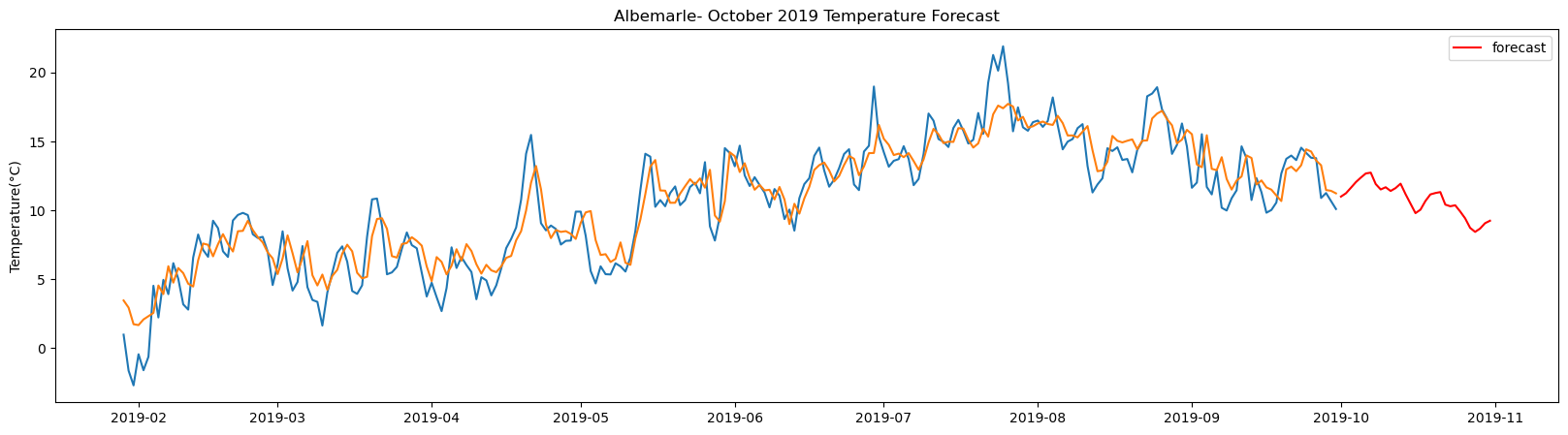
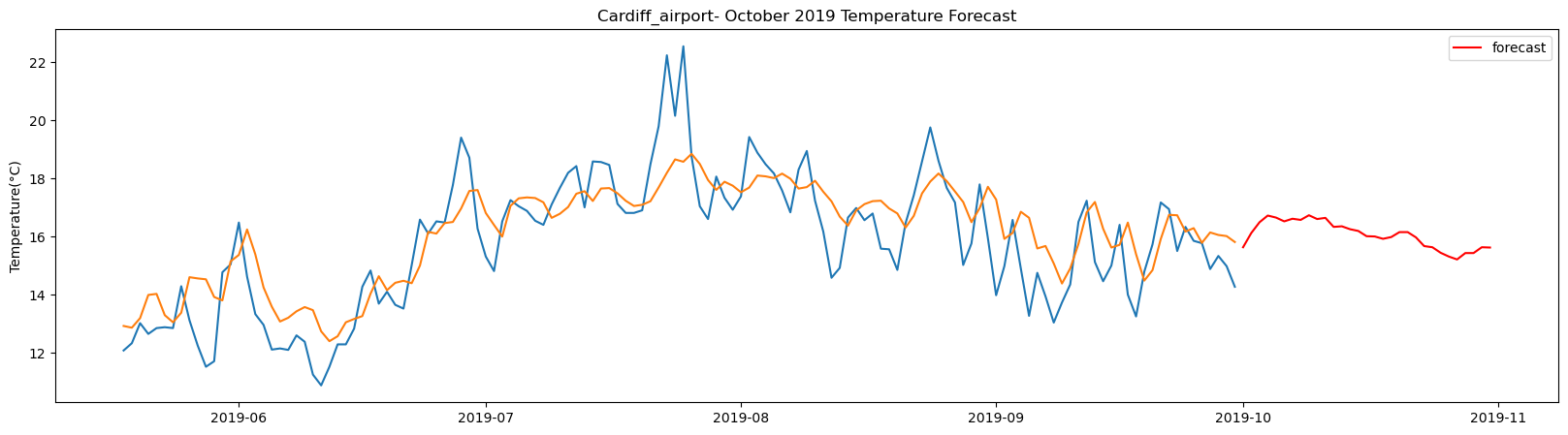
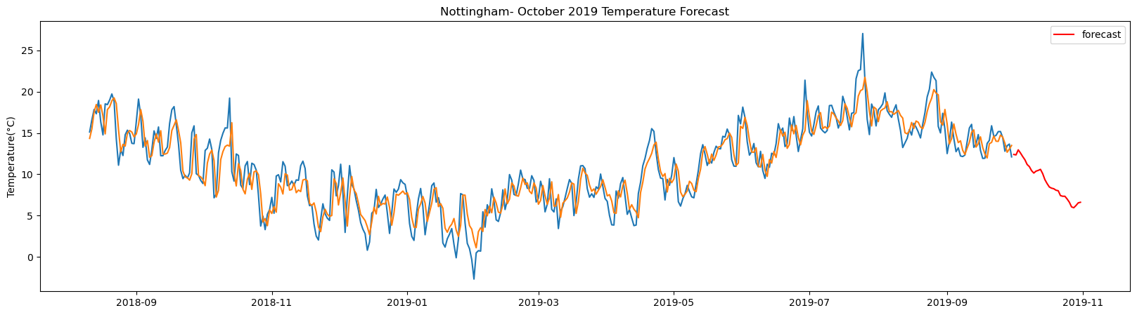
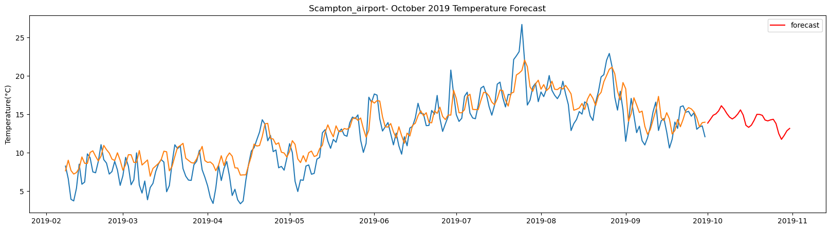
The result above returns the model metric of R-squared for the test data for each weather station followed by visualization of the actual past observations and the output predicted by the model for the same observation and the monthly forecast of October,2019. Here the past observed temperatures is in Blue, validation is in Orange and forecast is in Red. It is observed that the data is fitted reasonably with high accuracy for most of the stations.

Temperature forecasted by LSTM model

The forecasted temperature for the weather stations by the model is as follows:

# 30 days of forecast for October,2019 obtained from the LSTM model for each weather stations
lstm_prediction.head()

	Albemarle	Begwary	Birmingham_airport	Blackpool_airport	Boulmer_airport	Bournemouth_airport	BrizeNorton_airport	Cardiff_airport	Carlisle	Crosby	...	Norwich_airport	Nottingham	Plymouth_weatherstation	Rostherne	Scampton_airport	Shawbury_airport	Southend_on_Sea_AWS	Stansted_airport	Wittering_airport	Yeovilton_airport
2019-10-01	11.00	13.69	13.58	14.17	15.57	14.21	14.600000	15.630000	12.13	15.400000	...	14.170000	12.40	14.09	12.69	13.85	12.95	13.73	13.94	14.150000	13.77
2019-10-02	11.24	14.07	14.53	14.68	15.81	14.41	15.700000	16.120001	12.99	16.379999	...	15.000000	12.35	13.97	13.09	14.35	13.84	13.86	14.10	15.580000	13.99
2019-10-03	11.64	14.77	15.52	15.11	16.00	14.67	16.360001	16.490000	13.75	17.129999	...	15.780000	12.96	13.70	13.75	14.87	14.31	13.36	14.89	16.309999	13.91
2019-10-04	12.05	14.57	15.88	15.40	16.00	14.43	16.490000	16.719999	13.91	17.590000	...	15.730000	12.58	13.26	14.07	15.05	14.81	12.84	15.32	16.430000	13.84
2019-10-05	12.38	14.95	15.71	15.28	16.16	14.17	16.620001	16.650000	14.41	17.570000	...	16.110001	12.15	12.89	14.01	15.44	14.44	12.23	15.97	16.389999	13.18

5 rows × 29 columns

The table above gives the daily forecast for the month of October for each of the 29-location using LSTM. The columns indicate the location of the weather stations and the rows are the forecasted temperature in degree Celsius for each day of the month starting from 2019-10-01.

Support Vector Machine

Support Vector Machine was first proposed by Vladimir Vapnik as a binary linear classifier in 1963 which was further developed in 1992 to a non linear classifier. This algorithm classifies data by creating hyperplanes between different classes using the maximal margin method. The maximum margin represented as epsilon(ε) is the maximum separation distance(2ε) that can be achieved between the nearest data points of the two classes. These data points which are critical for the hyperplane are known as support vectors.

This study being a regression problem, here its regression variant also known as Support Vector Regression (SVR) is used, which was proposed in 1996 by Vapnik .et.al, suitable for regression in high dimensionality space. The algorithm uses the same maximal margin principle but instead of separating classes it creates a tube with a radius of epsilon(ε) to include the data points. The primary parameters for SVR are the kernel function and its coefficient required to map the data points to a higher dimension space, epsilon(ε) or tube radius, and C or cost as penalty.

In the second method this machine learning algorithm of Support Vector Regression (SVR) is applied to compare performances by the deep learning framework, since it is suitable for fitting high dimensional data with comparatively fewer samples.

Accordingly a function is first created which would first receive the time series data, followed by fitting it using the ML model and forecasting daily for the month of October, 2019.

The support vector regression here uses a radial basis function or rbf as the kernel, a moderate cost value of C=10 and an epsilon of 0.001. These are the critical parameters for the svr model, which can be further tuned for better result. This is then fitted on the train set and predicted on the test set, with accuracy of the fit measured in terms of R-squared.

# fitting & Validating using SVR
def fit_svr(X_train_tract1_array, y_train_tract1_array, X_test_tract1_array, y_test_tract1_array):
    model_svr = SVR(kernel='rbf', gamma='auto', tol=0.001, C=10.0, epsilon=0.001)
    model_svr.fit(X_train_tract1_array,y_train_tract1_array)
    y_pred_train_tract1 = model_svr.predict(X_train_tract1_array)
    y_pred_test_tract1 = model_svr.predict(X_test_tract1_array)        
    print('r-square_SVR_Test: ', round(model_svr.score(X_test_tract1_array,y_test_tract1_array),2))
    return model_svr, y_pred_test_tract1

The forecasted value on the test set using the fitted model is estimated and included with the actual observed temperatures set for visualization

# validation result  
def valid_result_svr(scaler, y_pred_test_tract1, station_value, split_row, lag):
    new_test_tract1 = station_value.iloc[split_row:]
    test_tract1_pred = new_test_tract1.iloc[lag:].copy()
    y_pred_test_tract1_transformed = scaler.inverse_transform([y_pred_test_tract1])
    y_pred_test_tract1_transformed_reshaped = np.reshape(y_pred_test_tract1_transformed,(y_pred_test_tract1_transformed.shape[1],-1))
    test_tract1_pred['Forecast'] = np.array(y_pred_test_tract1_transformed_reshaped)
    return test_tract1_pred

Once the model is validated the fitted model is used to forecast temperature for user input days using past data. This is also estimated using one day walk forward method as mentioned in case of LSTM.

# multi-step future forecast
def forecast_svr(X_test_tract1_array, days ,model_svr, lag, scaler):
    last_test_sample = X_test_tract1_array[-1]        
    X_last_test_sample = np.reshape(last_test_sample,(-1,X_test_tract1_array.shape[1]))        
    y_pred_last_sample = model_svr.predict(X_last_test_sample)                
    new_array = X_last_test_sample
    new_predict = y_pred_last_sample
    new_array = X_last_test_sample
    new_predict = y_pred_last_sample

    seven_days_svr=[]
    for i in range(0,days):               
            new_array = np.insert(new_array, 0, new_predict)                
            new_array = np.delete(new_array, -1)
            new_array_reshape = np.reshape(new_array, (-1,lag))                
            new_predict = model_svr.predict(new_array_reshape)
            temp_predict = scaler.inverse_transform([new_predict])
            seven_days_svr.append(temp_predict[0][0].round(2))
            
    return seven_days_svr

All the above methods are finally included in the main function which will take three input of the historical temperature data, number of lag data to be used and the number of days to be forecasted.

def england_temp_svr(all_station_temp, lag, days):     
    
    seven_day_forecast_svr = create_dates('2019-09-30',days)
    
    for i in range(len(all_station_temp.columns)):
        
        # preprocessing
        station_value, station_name = get_value_name(all_station_temp,i)       
        train_tract1, test_tract1, split_row = train_test_split(station_value, station_name, 0.80)              
        train_tract1_scaled_df, test_tract1_scaled_df, scaler = data_transformation(train_tract1,test_tract1)        
        train_tract1 = timeseries_feature_builder(train_tract1_scaled_df,lag+1)
        test_tract1 = timeseries_feature_builder(test_tract1_scaled_df, lag+1)        
        X_train_tract1_array, y_train_tract1_array, X_test_tract1_array, y_test_tract1_array = make_arrays(train_tract1,
                                                                                                           test_tract1)

        # SVR modeling
        model_svr, y_pred_test_tract1 = fit_svr(X_train_tract1_array, y_train_tract1_array,
                                                X_test_tract1_array, y_test_tract1_array)                       
        test_tract1_pred = valid_result_svr(scaler, y_pred_test_tract1, station_value, split_row, lag)        
        seven_days_svr = forecast_svr(X_test_tract1_array, days, model_svr, lag, scaler)            
        seven_day_forecast_svr[station_name] = np.array(seven_days_svr)        
        
        # plot result
        plt.figure(figsize=(20,5))
        plt.plot(test_tract1_pred)
        plt.plot(seven_day_forecast_svr[station_name], color='red', label='forecast') 
        plt.ylabel('Temperature(°C)')
        plt.legend(loc='upper right')
        plt.title(station_name + '- October 2019 Temperature Forecast')
        plt.show()    
        
    return(seven_day_forecast_svr)

The function is now called on the same temperature dataset and outputs are recorded. It is given three input: first the historic temperature dataset, the number of lagged terms to be used for prediction and finally the number of days of forecasting.

%%time
# Fitting and forecast using SVM
svr_prediction = england_temp_svr(all_station_temp, 365, 30)

Albemarle total samples:  3648
Training samples:  2918
Testing samples:  730
r-square_SVR_Test:  0.82

Begwary total samples:  3648
Training samples:  2918
Testing samples:  730
r-square_SVR_Test:  0.84

Birmingham_airport total samples:  2556
Training samples:  2044
Testing samples:  512
r-square_SVR_Test:  0.51

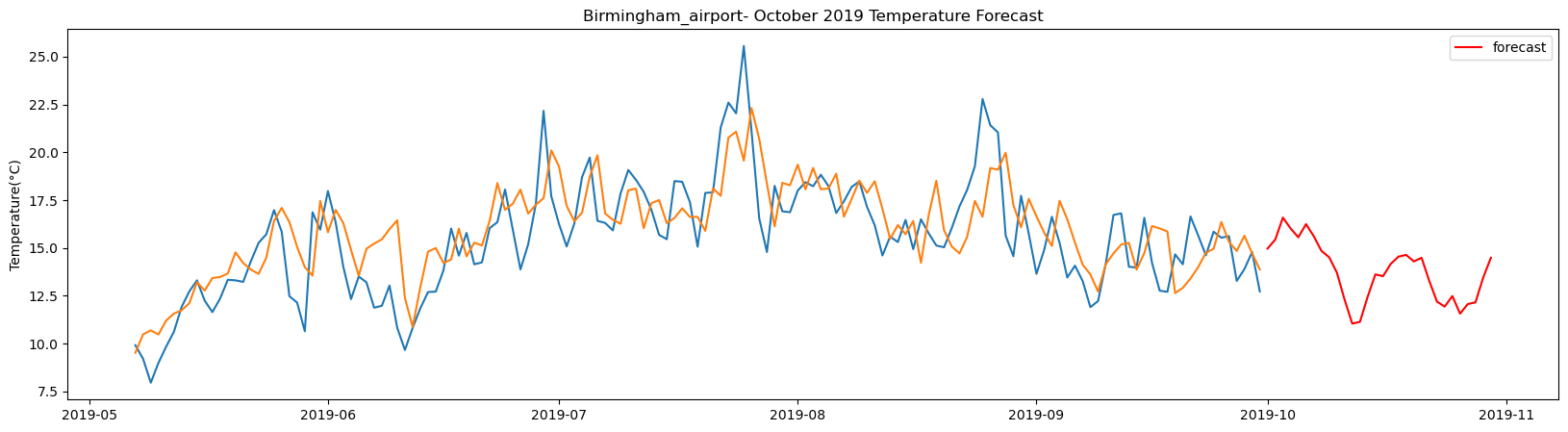
Blackpool_airport total samples:  3501
Training samples:  2800
Testing samples:  701
r-square_SVR_Test:  0.87

Boulmer_airport total samples:  5302
Training samples:  4241
Testing samples:  1061
r-square_SVR_Test:  0.83

Bournemouth_airport total samples:  3648
Training samples:  2918
Testing samples:  730
r-square_SVR_Test:  0.8

BrizeNorton_airport total samples:  5355
Training samples:  4284
Testing samples:  1071
r-square_SVR_Test:  0.87

Cardiff_airport total samples:  2556
Training samples:  2044
Testing samples:  512
r-square_SVR_Test:  0.61

Carlisle total samples:  3529
Training samples:  2823
Testing samples:  706
r-square_SVR_Test:  0.8

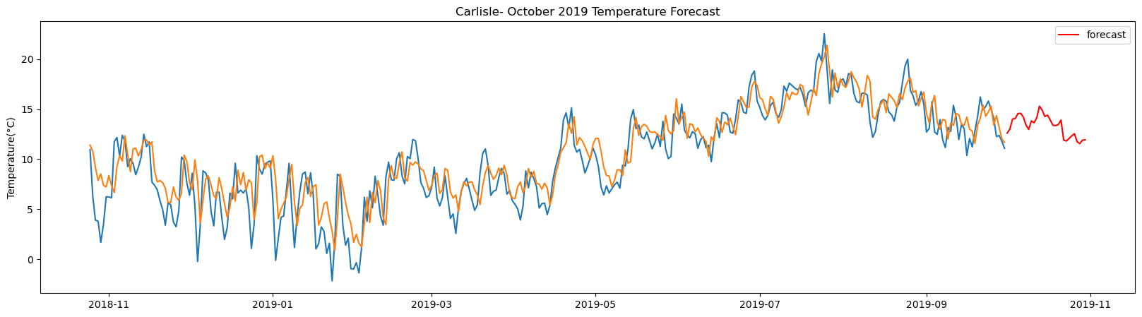
Crosby total samples:  3648
Training samples:  2918
Testing samples:  730
r-square_SVR_Test:  0.85

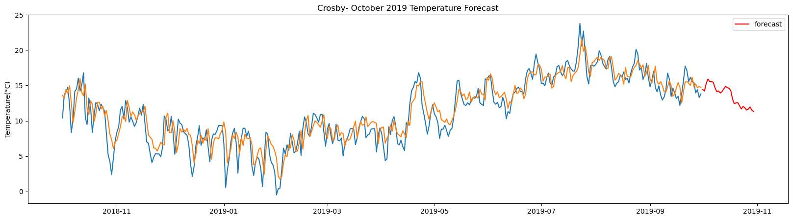
Culdrose_airport total samples:  2556
Training samples:  2044
Testing samples:  512
r-square_SVR_Test:  0.76

DurhamTeesValley_airport total samples:  2556
Training samples:  2044
Testing samples:  512
r-square_SVR_Test:  0.61

Exeter_airport total samples:  2556
Training samples:  2044
Testing samples:  512
r-square_SVR_Test:  0.5

Leconfield_airport total samples:  2555
Training samples:  2044
Testing samples:  511
r-square_SVR_Test:  0.51

SpadeadamKingwater_airport total samples:  2556
Training samples:  2044
Testing samples:  512
r-square_SVR_Test:  0.62

LeedsBradford_airport total samples:  2922
Training samples:  2337
Testing samples:  585
r-square_SVR_Test:  0.79

LondonCity_airport total samples:  2556
Training samples:  2044
Testing samples:  512
r-square_SVR_Test:  0.54

Lyneham_airport total samples:  5355
Training samples:  4284
Testing samples:  1071
r-square_SVR_Test:  0.87

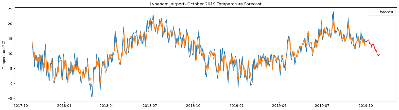
NewquayCornwall_airport total samples:  2556
Training samples:  2044
Testing samples:  512
r-square_SVR_Test:  0.64

Norwich_airport total samples:  2556
Training samples:  2044
Testing samples:  512
r-square_SVR_Test:  0.54

Nottingham total samples:  5355
Training samples:  4284
Testing samples:  1071
r-square_SVR_Test:  0.87

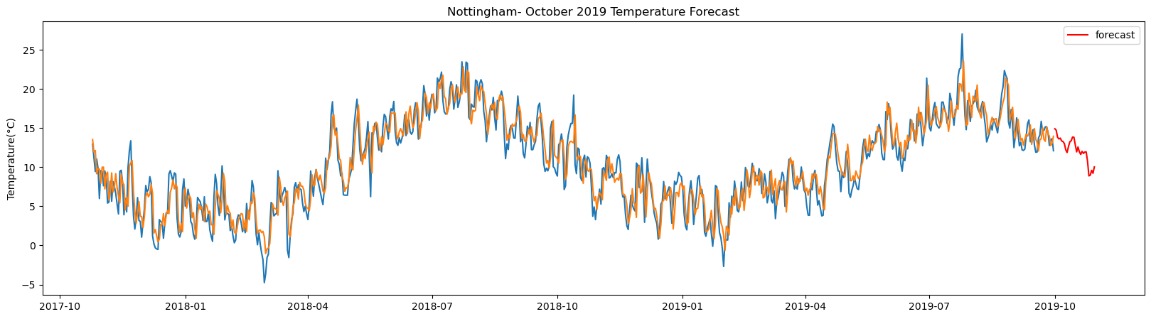
Plymouth_weatherstation total samples:  5355
Training samples:  4284
Testing samples:  1071
r-square_SVR_Test:  0.87

Rostherne total samples:  2495
Training samples:  1996
Testing samples:  499
r-square_SVR_Test:  0.5

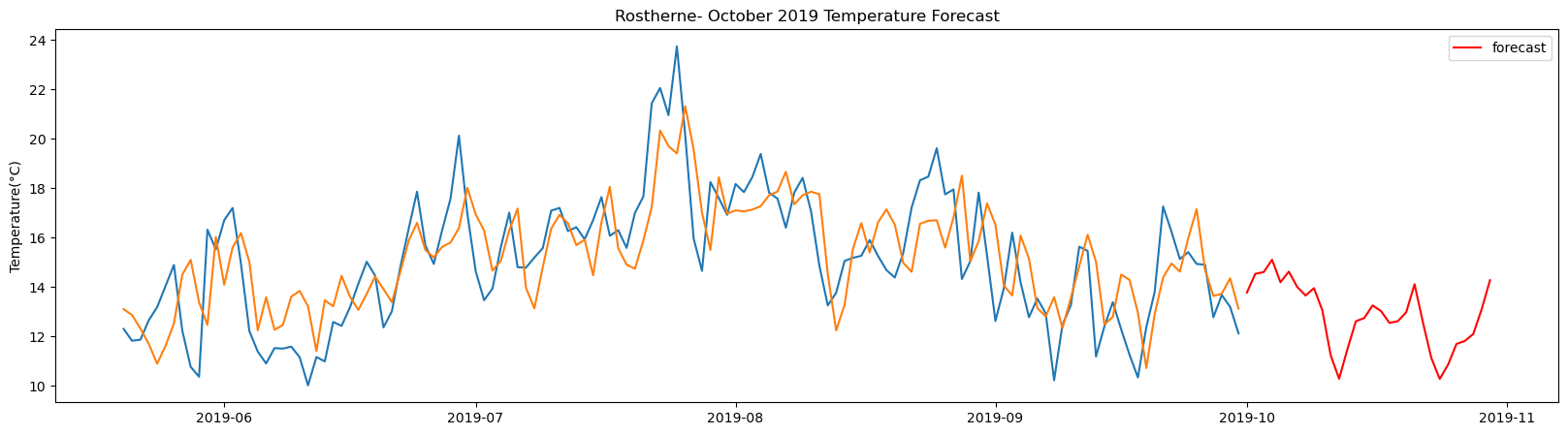
Scampton_airport total samples:  3543
Training samples:  2834
Testing samples:  709
r-square_SVR_Test:  0.79

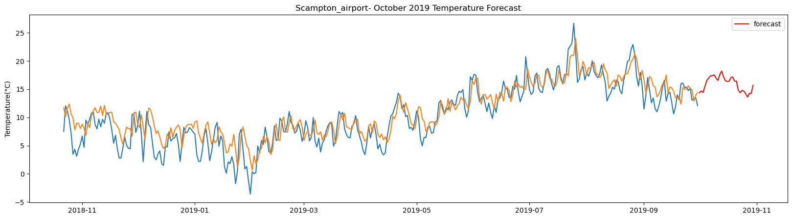
Shawbury_airport total samples:  5355
Training samples:  4284
Testing samples:  1071
r-square_SVR_Test:  0.84

Southend_on_Sea_AWS total samples:  3648
Training samples:  2918
Testing samples:  730
r-square_SVR_Test:  0.86

Stansted_airport total samples:  2556
Training samples:  2044
Testing samples:  512
r-square_SVR_Test:  0.53

Wittering_airport total samples:  5355
Training samples:  4284
Testing samples:  1071
r-square_SVR_Test:  0.87

Yeovilton_airport total samples:  5355
Training samples:  4284
Testing samples:  1071
r-square_SVR_Test:  0.84

CPU times: total: 3min 13s
Wall time: 3min 13s

In the above section the SVR model is trained on past time series data followed by forecasting temperature for the month of October,2019 for each of the stations. The results are plotted for each station with past observed temperatures in Blue, validation in Orange and forecast in Red. The validation closely matches the observed daily temperatures in most of the cases as also given by the test metrics of r-square with the highest values reaching up to 0.87 for the SVR model.

Temperature forecasted by SVR model

The output obtained by the above SVR model is visualized here which will now be processed to interpolate temperature for the whole of England.

# Daily forecast obtained from the SVR model for each of the weather stations
svr_prediction.head()

	Albemarle	Begwary	Birmingham_airport	Blackpool_airport	Boulmer_airport	Bournemouth_airport	BrizeNorton_airport	Cardiff_airport	Carlisle	Crosby	...	Norwich_airport	Nottingham	Plymouth_weatherstation	Rostherne	Scampton_airport	Shawbury_airport	Southend_on_Sea_AWS	Stansted_airport	Wittering_airport	Yeovilton_airport
2019-10-01	11.29	14.30	14.97	13.83	16.18	14.08	14.59	15.45	12.60	14.45	...	16.75	14.93	14.93	13.77	14.37	15.93	17.29	15.78	15.03	16.06
2019-10-02	9.78	13.69	15.44	14.48	16.82	15.33	14.74	15.87	13.01	14.21	...	16.98	14.74	14.80	14.53	14.70	15.38	15.99	16.52	14.19	15.77
2019-10-03	10.47	14.45	16.59	14.63	16.61	16.64	14.21	16.83	14.01	15.27	...	15.95	13.84	14.56	14.60	14.43	15.76	16.06	17.47	13.89	14.92
2019-10-04	11.32	14.62	16.02	14.73	15.88	17.02	14.25	17.63	14.07	15.91	...	15.76	13.62	14.09	15.10	15.55	16.40	16.43	16.42	13.45	15.71
2019-10-05	12.70	14.27	15.56	14.95	15.98	16.04	13.76	17.65	14.55	15.56	...	16.83	13.73	14.48	14.19	16.57	15.57	16.80	16.50	12.39	15.46

5 rows × 29 columns

Temperature Interpolation for England

Now the predictions obtained by the SVM method would be used for spatially mapping and estimating temperatures for the entire country for a certain day. Hence location of each weather station needs to be added to this table for the spatial operation. This is done in the following.

# Change station names to index
england_temp_forecast = svr_prediction.transpose()
# Make station names to a column
england_temp_forecast_station = england_temp_forecast.reset_index()
england_temp_forecast_station = england_temp_forecast_station.rename(columns={'index':'Station'})
# Join forecast temperature data to weather station location using the Staion column
predicted_temp_by_station = pd.merge(england_temp_forecast_station, england_weather_stations_layer_sdf, left_on='Station', right_on='Station', how='left')
predicted_temp_by_station.head()

	Station	2019-10-01 00:00:00	2019-10-02 00:00:00	2019-10-03 00:00:00	2019-10-04 00:00:00	2019-10-05 00:00:00	2019-10-06 00:00:00	2019-10-07 00:00:00	2019-10-08 00:00:00	2019-10-09 00:00:00	...	2019-10-25 00:00:00	2019-10-26 00:00:00	2019-10-27 00:00:00	2019-10-28 00:00:00	2019-10-29 00:00:00	2019-10-30 00:00:00	FID	Y	X	SHAPE
0	Albemarle	11.29	9.78	10.47	11.32	12.70	11.92	12.31	11.09	10.37	...	7.71	6.78	6.19	6.30	7.15	8.40	1	55.016667	-1.866667	{"x": -207796.38285121127, "y": 7365101.445978...
1	Begwary	14.30	13.69	14.45	14.62	14.27	14.83	14.79	14.78	13.96	...	14.66	13.47	12.06	12.06	11.56	11.54	2	52.216667	-0.483333	{"x": -53804.420512971476, "y": 6839396.777444...
2	Birmingham_airport	14.97	15.44	16.59	16.02	15.56	16.25	15.62	14.85	14.52	...	12.49	11.57	12.07	12.16	13.45	14.49	3	52.45	-1.733333	{"x": -192953.78400456344, "y": 6881903.804921...
3	Blackpool_airport	13.83	14.48	14.63	14.73	14.95	15.49	15.65	14.91	14.62	...	11.62	10.88	11.11	10.96	11.32	12.13	4	53.766667	-3.033333	{"x": -337669.1220358203, "y": 7126089.0211904...
4	Boulmer_airport	16.18	16.82	16.61	15.88	15.98	15.66	15.07	15.07	16.59	...	14.46	14.66	15.04	16.14	17.12	16.28	5	55.4203	-1.5997	{"x": -178077.78942199165, "y": 7443868.808735...

5 rows × 35 columns

Result Visualization

Now the table above gives the daily temperature forecast for the month of October,2019 for all the 29 weather stations in England, with location of each station. Out of these predictions the first day of October is selected for creating a probable temperature surface for the entire country.

# Select the first day out 
oct1st_temp = predicted_temp_by_station.iloc[:, [0,1,33,32]]
oct1st_temp = oct1st_temp.rename(columns={oct1st_temp.columns[1]:'temp_pred'})
oct1st_temp.head()

	Station	temp_pred	X	Y
0	Albemarle	11.29	-1.866667	55.016667
1	Begwary	14.30	-0.483333	52.216667
2	Birmingham_airport	14.97	-1.733333	52.45
3	Blackpool_airport	13.83	-3.033333	53.766667
4	Boulmer_airport	16.18	-1.5997	55.4203

The data is now converted into a spatial data frame in the following.

# convert dataframe to a spatial dataframe
sdf = oct1st_temp.spatial.from_xy(df=oct1st_temp, sr=4326, x_column='X', y_column='Y')
# create feature layer from the spatial dataframe
oct1st_temp_points = gis.content.import_data(sdf, title='eng_temp_points')

oct1st_temp_points

eng_temp_points

Feature Layer Collection by MMajumdar_geosaurus
Last Modified: November 27, 2024
0 comments, 0 views

The interpolate_points method from the ArcGIS API for Python allows us to predict values at new locations based on measurements from a collection of points. The method takes point data with values at each point and returns areas classified by predicted values.

For example, we are using interpolate_points tool to estimate temperature of England. The input parameters required for the tool are:

input_layer: feature layer having the predicted temperature for all the weather stations
interpolate_options specify the speed v/s accuracy on a range of 1 to 9 with 9 as the maximum accuracy
field indicates the column name in the feature layer which has the predicted temperatures
bounding_polygon_layer here is the England boundary shapefile which sets the boundary within which the spatial interpolation would be estimated
output_name the name of the resulting output interpolated surface.

# Interpolate the predicted temperature data to create forecast surface for England
oct1st_temp_surface = interpolate_points(oct1st_temp_points, 
                                         interpolate_option=9,                                         
                                         field='temp_pred', 
                                         bounding_polygon_layer=england_boundary_layer,
                                         output_name='Interpolated Temperature'+ str(dt.now().microsecond))

{"cost": 0.334}

oct1st_temp_surface

Interpolated_Temperature460501

Feature Layer Collection by MMajumdar_geosaurus
Last Modified: November 27, 2024
0 comments, 0 views

# Plot the interpolated temperature surface
eng_interpolated_temp = gis.map('England')
eng_interpolated_temp.basemap.basemap = 'topo-vector'
eng_interpolated_temp.content.add(oct1st_temp_surface)
eng_interpolated_temp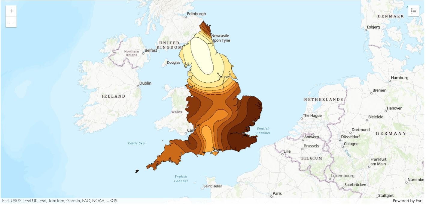

eng_interpolated_temp.zoom = 6
eng_interpolated_temp.legend.enabled = True

The interpolated forecast temperature surface above for England shows that temperature gradually increases from the northern to the southern part of the country, and ranges from a minimum of 9.5 degrees to a maximum of 17.43 degree Celsius respectively, with two distinct zones dividing the country. Lower temperatures are prevalent in the interior part of the country compared to the coastal belts, with London falling in the maximum temperature zone. This is expected since coastal regions are usually warmer than inland areas due to different climatic conditions.

Conclusion

In this notebook, a timeseries temperature dataset was used to predict daily temperature for England for the month of October using historic data from 29 weather stations. Two methods were used for the study — first a deep learning framework of LSTM was used followed by a machine learning method of Support Vector Regression. Both the models were able to model the data relatively well as evident from the high accuracy obtained for both train and test set. However, the SVM model was consistently performing better than the LSTM model with higher accuracy. Some instances of low accuracy for both the models were caused for certain stations due to less training data points available.

Similarly, interesting differences were observed while forecasting daily temperatures using the two models. Here the SVR model was able to capture the daily fluctuations in greater detail which looked more real compared to the forecast returned by the LSTM model, as observed from the forecast plots. Besides, the total run time for the SVR model for fitting the data was only a few minutes and was far less than the time taken by the LSTM model, which was training for 100 epochs for each station.

Finally, the sample shows how deep learning or machine learning models could be combined with spatial tools in ArcGIS to process timeseries data and produce meaningful results that could be valuable for various industry verticals.

Summary of methods used

Method	Question	Examples
interpolate_points	What is the value of any points located between other given points?	Predicting temperature at any intermediate location based on measurement from surrounding station

Data resources

Shapefile	Source	Link
england_border	Counties and Unitary Authorities (December 2016) Full Clipped Boundaries in England and Wales	https://data.gov.uk
england_weather_stations	Weather for 243 countries of the world	https://rp5.ru/Weather_in_the_world
table(england historic weather data)	Weather for 243 countries of the world	https://rp5.ru/Weather_in_the_world

Articles	Source	Link
LONG SHORT-TERM MEMORY	Neural Computation 9(8):1735{1780, 1997	http://www.bioinf.jku.at/publications/older/2604.pdf
Support Vector Regression Machines	Bell Labs and Monmouth University Department of Electronic Engineering	https://papers.nips.cc/paper/1238-support-vector-regression-machines.pdf