Using the map widget
The GIS object includes a map widget for displaying geographic locations, visualizing GIS content, and displaying the results of your analysis. To use the map widget, call gis.map() and assign it to a variable that you will then be able to query to bring up the widget in the notebook:
import arcgis
from arcgis.gis import GIS
# Create a GIS object, as an anonymous user for this example
gis = GIS()
Create a map widget
Passing an argument to the location parameter initializes the widget to a particular place and configures an extent.
map1 = gis.map(
    location="Redlands, CA"
)
map1
Map Buttons
Now that we have created a map view, let us explore the default buttons enabled on the widget:
1. Zoom in
Click the "+" sign shown on the top left corner of the widget (marked as button #1 in previous map output) to zoom into a larger scale. Users can either manually zoom into a desired level of detail or set the zoom levels to an assigned number, which we will elaborate on in the next section.
2. Zoom out
Click the "-" sign shown on the top left corner of the widget (marked as button #2 in previous map output) to zoom out to a smaller scale. Users can either manually zoom out to a desired level of details, or set the zoom levels to an assigned number, which we will elaborate on in the next section.
Note: You can scroll with a mouse or touchpad to zoom in and out as well.
You can click and drag on the widget to pan across the map.
Create a scene widget
scene1 = gis.map(
    location="Redlands, CA",
    mode="3D"
)
scene1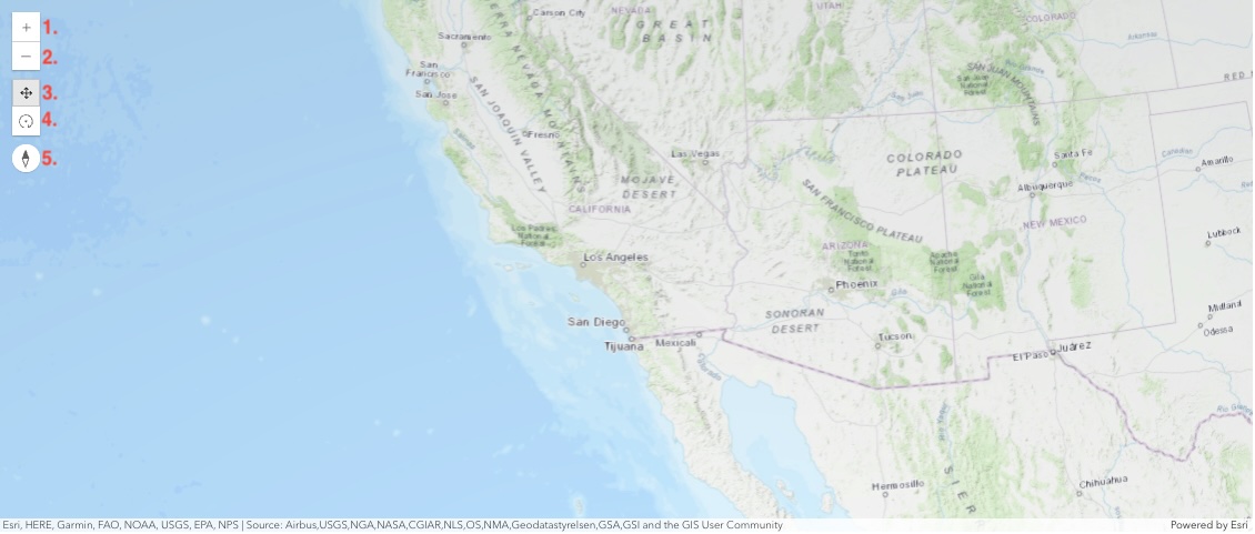
Scene Buttons
Now that we have created a scene view, let us explore the default buttons enabled on the widget:
1. Zoom in
Click the "+" sign shown on the top left corner of the widget (marked as button #1 in previous map output) to zoom in on details of the scene. Users can either zoom into a desired level of detail with the buttons or set the zoom levels to an assigned number, which we will elaborate on in the next section.
2. Zoom out
Click the "-" sign shown on the top left corner of the widget (marked as button #2 in previous map output) to zoom out to a smaller-scale display of the map. Users can either zoom out with the button to a desired level of details, or set the zoom levels to an assigned number, which we will elaborate on in the next section.
Note: You can scroll with a mouse or touchpad to zoom in and out as well.
3. Pan
Click the button, then click on the scene while dragging in the direction you want to move across the screen. (You can also use the arrow keys on your keyboard).
4. Rotate
Click the button, then click on the scene while dragging in the direction you want to rotate and tilt the camera.
5. Compass
Click the button to orient the scene to North. As you move around the scene, the compass marker moves to reflect the orientation.
See Scene navigation for more details.
Properties of the map widget
The map widget has several properties that you can query and set, such as its zoom level, extent, center, scale and rotation amongst others. It also has properties that initialize other classes, such as basemap, which allow for additional management capabilities of the map. Type the map variable name, a dot, then hit the tab key in a notebook to see options.
Zoom Level and Rotation
map2 = gis.map(location="Rangoon")
map2
note: Screenshot above will appear after setting the rotation property 3 cells after initially rendering the map.
map2.zoom11.0
Assigning a value to the zoom property will update the widget, which is equivalent to manually clicking the zoom button either in or out as many times as the difference between the current zoom level and the number you enter.
map2.zoom = 9You can also set the rotation property for the map.
map2.rotation = 45Your notebook can have as many of these widgets as you wish. Let's create another map widget and modify some of its properties.
Map Center
Let's examine the map as it comes in with the default properties, and examine the center property to reveal the coordinates of the middle of the map.
map3 = gis.map()
map3
note: The screenshot above will display after running the 10 cells below culminating with setting the basemap.
map3.center[-95.22142011666926, 38.14549630928053]
note: The coordinates are reported as a list in [ longitude, latitude ] format.
If you know the latitude and longitude of a place of interest, you can assign a list to the center property to focus the map on that location. For instance, we can set the center of our map to be the coordinates (in [latitude, longitude] format using in the WGS 84 Spatial Reference) of Oklahoma City:
map3.center = [35.4666492, -97.5229713]Set the zoom to a larger scale to verify
map3.zoom = 10Extent
You can use geocoding to get the coordinates of different places and use those coordinates to drive the extent property. Geocoding converts place names to coordinates and can be implemented by using the geocode() function in the arcgis.geocode module.
Let's geocode "Disneyland, CA" and set the map's extent to the geocoded location's extent:
from arcgis.geocoding import geocode, get_geocodersLet's also find out what the default geocoder is for an anonymous connection, and return the spatial reference used by the geocoder:
anon_gc = get_geocoders(gis)
anon_gc
[<Geocoder url:"https://geocode.arcgis.com/arcgis/rest/services/World/GeocodeServer">]
anon_gc[0].properties["spatialReference"]{'wkid': 4326, 'latestWkid': 4326}Now let's geocode a particular location and then add the spatial reference to it for setting the extent:
location = geocode('Disneyland, CA', max_locations=1)[0]
location["extent"]
{'xmin': -117.9239585,
'ymin': 33.8049461,
'xmax': -117.9139585,
'ymax': 33.8149461}location["extent"].update({
"spatialReference": {
"wkid": 4326
}
}
)location["extent"]{'xmin': -117.9239585,
'ymin': 33.8049461,
'xmax': -117.9139585,
'ymax': 33.8149461,
'spatialReference': {'wkid': 4326}}map3.extent = location['extent']Basemap
ArcGIS Living Atlas of the World is an evolving collection of authoritative, curated, ready-to-use global geographic information from Esri and the GIS user community. One of the more popular types of content from the Living Atlas is basemaps. Basemaps are layers on your which serve to reference all the operational layers displayed on top of them. Basemaps typically span the full extent of the world and provide context to your GIS layers. It helps viewers understand where each feature is located as they pan and zoom to various extents.
When you create a new map or scene, you can choose which basemap you want from the basemap gallery in the Map Viewer. By default, the basemap gallery for your organization is a pre-configured collection from Esri using the Living Atlas. There are many more Living Atlas basemaps to choose from, and you can create your own custom basemap gallery with the ones you like. Learn more on this here.
As an administrator of your organization, you can change which basemaps your organization uses by creating a custom basemap gallery. The custom gallery can include a combination of your own basemaps, plus Living Atlas basemaps. In a nutshell, the steps to create a custom basemap gallery are as follows:
- Create a group for your custom basemap gallery.
- Add maps you want to use as basemaps to the group.
- Set the group as your organization’s basemap gallery.
These steps are detailed in the Create a custom basemap gallery for your organization blog. After step one is done, users can move forward to :
When your gis connection is created, the basemap property accesses a BasemapManager, and the basemaps property will reveal the basemaps available to the current user. In this case, we're using an anonymous user in the Web GIS, so the Map will be displayed with default themes.
note: Basemaps prefaced with
arcgis-require an account to access.
When signing onto your own organization, the properties would display your own customized options if set.
Your map can have a number of different basemaps. To see what basemaps are included with the widget, query the basemaps property on the BasemapManager:
map3.basemap.basemaps['satellite', 'hybrid', 'terrain', 'oceans', 'osm', 'dark-gray-vector', 'gray-vector', 'streets-vector', 'topo-vector', 'streets-night-vector', 'streets-relief-vector', 'streets-navigation-vector', 'arcgis-imagery', 'arcgis-imagery-standard', 'arcgis-imagery-labels', 'arcgis-light-gray', 'arcgis-dark-gray', 'arcgis-navigation', 'arcgis-navigation-night', 'arcgis-streets', 'arcgis-streets-night', 'arcgis-streets-relief', 'arcgis-topographic', 'arcgis-oceans', 'osm-standard', 'osm-standard-relief', 'osm-streets', 'osm-streets-relief', 'osm-light-gray', 'osm-dark-gray', 'arcgis-terrain', 'arcgis-community', 'arcgis-charted-territory', 'arcgis-colored-pencil', 'arcgis-nova', 'arcgis-modern-antique', 'arcgis-midcentury', 'arcgis-newspaper', 'arcgis-hillshade-light', 'arcgis-hillshade-dark', 'arcgis-human-geography', 'arcgis-human-geography-dark']
Use the basemap property to return a dictionary representation of the current basemap:
map3.basemap.basemap{'baseMapLayers': [{'id': '1916d180fe2-layer-0',
'layerType': 'ArcGISTiledMapServiceLayer',
'opacity': 1.0,
'refreshInterval': 0.0,
'title': 'b6dbd29',
'url': 'https://services.arcgisonline.com/ArcGIS/rest/services/World_Topo_Map/MapServer',
'visibility': True}],
'title': 'Topographic'}You can assign any one of the supported basemaps to the basemap property to change the basemap. For instance, you can change the basemap to the satellite basemap as below:
map3.basemap.basemap = "satellite"Properties of the Scene widget
The map widget also includes support for a 3D mode! You can specify the mode parameter either through gis.map(mode="foo") or by setting the mode property of any initiated map object. Run the following cell:
usa_scene = gis.map(
    location="Omaha, NE",
    mode="3D"
)
usa_scene
Note: The screenshot above will appear after running the cells below culminating with setting the heading
Zoom
usa_scene.zoom6.0
Set the zoom to a small scale to observe the 3D mode more readily
usa_scene.zoom = 3Scene center
usa_scene.center[-95.93719500000002, 41.25883177381306]
Set the center to Seattle
usa_scene.center = [47.6061, -122.3328]Camera, tilt, and heading
You can pan a scene by clicking-and-dragging with the left mouse button, and you can zoom with the mouse wheel. Clicking-and-dragging with the right mouse button modifies the tilt field and the heading field. You can access these properties directly from the scene object, or get them from the camera property. The camera property of a scene returns a dictionary with the following keys:
position- the coordinate position of the camera including the elevation and a spatial referencetiltis a number from 0-90, with 0 representing a top-down 'birds-eye' view, while 90 represents being completely parallel to the ground, facing the horizonheadingis a number between 0 and 360 and indicates the direction the camera is pointing as a compass bearing: 0 is facing north, 90 is facing east, and 180 is facing south.
The position of the camera has impact on the view if you change the tilt and heading values. Use the zoom in, zoom out, rotate, and pan buttons to change the view of the scene, then print out the camera properties to see how the balues change>
usa_scene.camera{'position': {'spatialReference': {'latestWkid': 3857, 'wkid': 102100},
'x': -8734468.751698757,
'y': 1138794.7868943617,
'z': 4032935.8785236254},
'heading': 359.6662172401241,
'tilt': 30.65604577416708}usa_scene.tilt30.65604577416708
usa_scene.tilt = 42It's important to note that a map uses rotation to specify the number of angles clockwise from due north, while a scene uses the heading property. See the ArcGIS Pro Camera properties documentation for more details.
usa_scene.heading359.66661270395485
usa_scene.heading = 60Using multiple map widgets
Demo: Stacking maps using HBox and VBox
One commonly adopted workflow for creating multiple widgets in the same notebook is to embed Python API map widgets within HBox and VBox. First, let's walk through an example of displaying Landsat imagery of two different dates side by side using an HBox structure:
import warnings
warnings.filterwarnings("ignore", "Warning")
from arcgis.gis import GIS
gis = GIS(profile="your_online_profile")Search for a satellite imagery item:
landsat_item = gis.content.search("landsat Multispectral tags:'Landsat on AWS', 'landsat 8', 'Multispectral', 'Multitemporal', 'imagery', 'temporal', 'MS'", "Imagery Layer", outside_org=True)[0]
landsat = landsat_item.layers[0]
landsat
import pandas as pd
import datetime as dt
from ipywidgets import *
from arcgis import geocode
from arcgis.geometry.filters import intersects
aoi = {'xmin': -117.58051663099998,
'ymin': 33.43943880400006,
'xmax': -114.77651663099998,
'ymax': 36.243438804000064,
'spatialReference': {'latestWkid': 4326, 'wkid': 102100},}selected1 = landsat.filter_by(where="(Category = 1) AND (CloudCover <=0.10)",
time=[dt.datetime(2017, 11, 15), dt.datetime(2018, 1, 1)],
geometry=intersects(aoi))
df = selected1.query(out_fields="AcquisitionDate, GroupName, CloudCover, DayOfYear",
order_by_fields="AcquisitionDate").sdf
df['AcquisitionDate'] = pd.to_datetime(df['AcquisitionDate'], unit='ms')
df.tail(5)| OBJECTID | AcquisitionDate | GroupName | CloudCover | DayOfYear | SHAPE | |
|---|---|---|---|---|---|---|
| 17 | 2077276 | 2017-12-27 18:21:56 | LC08_L1TP_040035_20171227_20200902_02_T1_MTL | 0.0033 | 35 | {"rings": [[[-12818204.659699999, 4395823.9407... |
| 18 | 2077299 | 2017-12-27 18:22:20 | LC08_L1TP_040036_20171227_20200902_02_T1_MTL | 0.0023 | 36 | {"rings": [[[-12866539.864599999, 4199117.8993... |
| 19 | 2077322 | 2017-12-27 18:22:44 | LC08_L1TP_040037_20171227_20200902_02_T1_MTL | 0.0025 | 37 | {"rings": [[[-12913258.506099999, 4005782.8035... |
| 20 | 2072419 | 2017-12-29 18:09:58 | LC08_L1TP_038036_20171229_20200902_02_T1_MTL | 0.0004 | 36 | {"rings": [[[-12522415.1111, 4199148.978100002... |
| 21 | 2072442 | 2017-12-29 18:10:21 | LC08_L1TP_038037_20171229_20200902_02_T1_MTL | 0.0014 | 37 | {"rings": [[[-12569056.4399, 4005554.541000001... |
selected2 = landsat.filter_by(where="(Category = 1) AND (CloudCover <=0.10)",
                              time=[dt.datetime(2021, 11, 15), dt.datetime(2022, 1, 1)],
                              geometry=intersects(aoi))

df = selected2.query(out_fields="AcquisitionDate, GroupName, CloudCover, DayOfYear",
                     order_by_fields="AcquisitionDate").sdf
df['AcquisitionDate'] = pd.to_datetime(df['AcquisitionDate'], unit='ms')
df.tail(5)| OBJECTID | AcquisitionDate | GroupName | CloudCover | DayOfYear | SHAPE | |
|---|---|---|---|---|---|---|
| 9 | 3385195 | 2021-11-29 18:16:44 | LC08_L1TP_039037_20211129_20211209_02_T1_MTL | 0.0013 | 37 | {"rings": [[[-12738717.156100001, 4005622.7378... |
| 10 | 4408428 | 2021-12-05 18:28:20 | LC09_L1TP_041035_20211205_20230505_02_T1_MTL | 0.0651 | 35 | {"rings": [[[-12990717.9388, 4395637.728600003... |
| 11 | 3385196 | 2021-12-15 18:16:43 | LC08_L1TP_039037_20211215_20211223_02_T1_MTL | 0.0052 | 37 | {"rings": [[[-12739407.4636, 4005732.446599997... |
| 12 | 4402130 | 2021-12-16 18:10:04 | LC09_L1TP_038036_20211216_20230504_02_T1_MTL | 0.0889 | 36 | {"rings": [[[-12519642.727400001, 4199040.7172... |
| 13 | 4402131 | 2021-12-16 18:10:28 | LC09_L1TP_038037_20211216_20230504_02_T1_MTL | 0.001 | 37 | {"rings": [[[-12566514.715599999, 4005583.7243... |
def side_by_side(address, layer1, layer2):

    satmap1 = gis.map(
        location=address
    )
    satmap1.content.add(layer1)

    satmap2 = gis.map(
        location=address
    )
    satmap2.content.add(layer2)

    satmap1.layout=Layout(flex='1 1', padding='6px', height='450px')
    satmap2.layout=Layout(flex='1 1', padding='6px', height='450px')

    box = HBox([satmap1, satmap2])
return boxside_by_side("San Bernadino County, CA", selected1, selected2)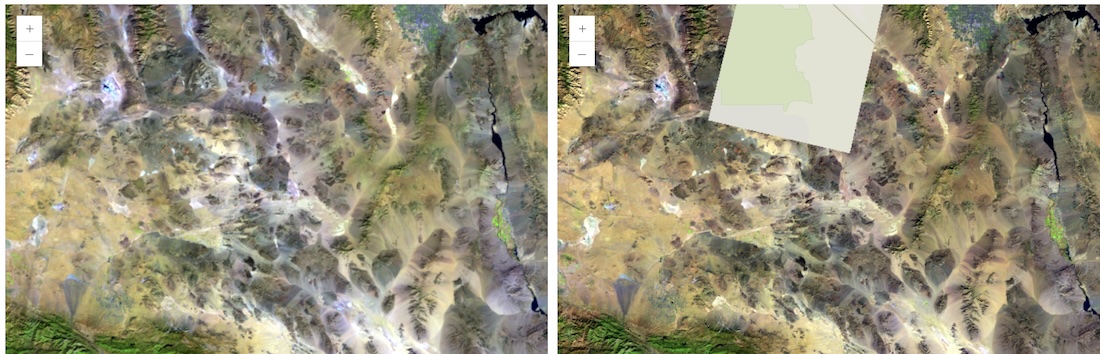
Demo: Synchronizing nav between multiple widgets
A side-by-side display of two maps is great for users wanting to explore the differences between two maps. However, if one map gets dragged or panned, the other map is not following the movements automatically. The methods sync_navigation and unsync_navigation can be introduced to resolve this. With these methods, we can modify the previous example to have the maps in sync.
def side_by_side2(address, layer1, label1, layer2, label2):
    # Create the first map
    satmap1 = gis.map(location=address)
    satmap1.content.add(layer1)

    # Create the second map
    satmap2 = gis.map(location=address)
    satmap2.content.add(layer2)

    # sync maps' navigation
    satmap1.sync_navigation(satmap2)

    # Create VBoxes for each map and label
    box1 = VBox([Label(label1), satmap1], layout=Layout(width='50%'))
    box2 = VBox([Label(label2), satmap2], layout=Layout(width='50%'))

    # Place the VBoxes side by side using an HBox
    hbox = HBox([box1, box2])

    # Display the HBox
display(hbox)side_by_side2("San Bernardino County, CA", selected1, 'Dec 2017', selected2, 'Dec 2021')
Demo: The synced display of 4 maps
Now let's sync the display of 4 maps:
selected1r = landsat.filter_by(where="(Category = 1) AND (CloudCover <=0.10)",
                               time=[dt.datetime(2018, 11, 15), dt.datetime(2019, 1, 1)],
                               geometry=intersects(aoi))

df = selected1r.query(out_fields="AcquisitionDate, GroupName, CloudCover, DayOfYear",
                     order_by_fields="AcquisitionDate").sdf
df['AcquisitionDate'] = pd.to_datetime(df['AcquisitionDate'], unit='ms')
df.tail(5)| OBJECTID | AcquisitionDate | GroupName | CloudCover | DayOfYear | SHAPE | |
|---|---|---|---|---|---|---|
| 4 | 1683891 | 2018-12-16 18:09:40 | LC08_L1TP_038036_20181216_20200830_02_T1_MTL | 0.0311 | 36 | {"rings": [[[-12518740.9842, 4199058.405000001... |
| 5 | 1687739 | 2018-12-23 18:15:27 | LC08_L1TP_039035_20181223_20200830_02_T1_MTL | 0.0453 | 35 | {"rings": [[[-12642295.304499999, 4395699.8553... |
| 6 | 1690955 | 2018-12-30 18:21:38 | LC08_L1TP_040035_20181230_20200829_02_T1_MTL | 0.0548 | 35 | {"rings": [[[-12814406.3816, 4395749.071999997... |
| 7 | 1690978 | 2018-12-30 18:22:02 | LC08_L1TP_040036_20181230_20200830_02_T1_MTL | 0.0085 | 36 | {"rings": [[[-12862669.9624, 4198971.424900003... |
| 8 | 1691001 | 2018-12-30 18:22:26 | LC08_L1TP_040037_20181230_20200830_02_T1_MTL | 0.0011 | 37 | {"rings": [[[-12909449.0056, 4005655.638700001... |
selected2l = landsat.filter_by(where="(Category = 1) AND (CloudCover <=0.10)",
                              time=[dt.datetime(2020, 11, 15), dt.datetime(2021, 1, 1)],
                              geometry=intersects(aoi))

df = selected2l.query(out_fields="AcquisitionDate, GroupName, CloudCover, DayOfYear",
                     order_by_fields="AcquisitionDate").sdf
df['AcquisitionDate'] = pd.to_datetime(df['AcquisitionDate'], unit='ms')
df.tail(5)| OBJECTID | AcquisitionDate | GroupName | CloudCover | DayOfYear | SHAPE | |
|---|---|---|---|---|---|---|
| 14 | 338139 | 2020-12-05 18:10:33 | LC08_L1TP_038037_20201205_20210313_02_T1_MTL | 0.001 | 37 | {"rings": [[[-12590665.892099999, 3909761.2709... |
| 15 | 2952645 | 2020-12-10 18:28:17 | LC08_L1TP_041035_20201210_20210313_02_T1_MTL | 0.0963 | 35 | {"rings": [[[-12988587.3908, 4395753.784199998... |
| 16 | 356604 | 2020-12-19 18:22:05 | LC08_L1TP_040035_20201219_20210310_02_T1_MTL | 0.006 | 35 | {"rings": [[[-12816854.251699999, 4395799.5128... |
| 17 | 356626 | 2020-12-19 18:22:29 | LC08_L1TP_040036_20201219_20210310_02_T1_MTL | 0.0026 | 36 | {"rings": [[[-12865073.5445, 4199098.650499999... |
| 18 | 356648 | 2020-12-19 18:22:53 | LC08_L1TP_040037_20201219_20210310_02_T1_MTL | 0.0004 | 37 | {"rings": [[[-12911955.1563, 4005769.613499999... |
def side_by_side3(address, layers_list, labels_list):
    [layer1, layer2, layer3, layer4] = layers_list
    [label1, label2, label3, label4] = labels_list

    # Location can be an address string or coordinates
    location = address

    # Create the maps
    satmap1 = gis.map(location=location)
    satmap1.content.add(layer1)

    satmap2 = gis.map(location=location)
    satmap2.content.add(layer2)

    satmap3 = gis.map(location=location)
    satmap3.content.add(layer3)

    satmap4 = gis.map(location=location)
    satmap4.content.add(layer4)

    # Create VBox for each map and its label
    box1 = VBox([Label(label1), satmap1], layout=Layout(width='50%'))
    box2 = VBox([Label(label2), satmap2], layout=Layout(width='50%'))
    box3 = VBox([Label(label3), satmap3], layout=Layout(width='50%'))
    box4 = VBox([Label(label4), satmap4], layout=Layout(width='50%'))

    # Create two HBoxes to hold two maps each
    hbox_top = HBox([box1, box2])
    hbox_bottom = HBox([box3, box4])

    # Set layout preferences
    hbox_layout = Layout(justify_content='space-around')
    hbox_top.layout = hbox_layout
    hbox_bottom.layout = hbox_layout

    # Sync all maps
    satmap1.sync_navigation(satmap2)
    satmap1.sync_navigation(satmap3)
    satmap1.sync_navigation(satmap4)

    # Combine the HBoxes into a VBox to display as a 2x2 grid
    return VBox([hbox_top, hbox_bottom])
# Example usage:
side_by_side3(
  "San Bernardino County, CA",
  [selected1, selected1r, selected2l, selected2],
  ['Dec 2017', 'Dec 2018', 'Dec 2020', 'Dec 2021']
)
Dragging and panning onto any of these 4 maps will lead to synchronous movements of the other three maps, which means that the map center, zoom levels, and extent of these maps will always stay the same. This is one of the biggest advantages of sync_navigation().
Conclusion
In Part 2 of the guide series, we have talked about the use of map widgets, including buttons, features, and properties, and have seen three examples of displaying multiple map widgets in a group view using HBox and VBox. In the next chapter, we will discuss how to visualize spatial data on the map widget.