Summarize data using binning functions

Spatial binning functions (spatial aggregation) give you a way to summarize spatial data for visualization and analysis. Summarizing spatial data is useful for both visualization of large datasets, and analysis. Many GeoAnalytics Engine tools use binning functionality as a core component of analysis, such as Summarize Within and Aggregate Points. In this tutorial you will learn how to use spatial binning functions such as ST_SquareBin, ST_SquareBins, ST_HexBin, ST_HexBins, ST_H3Bin, ST_H3Bins, ST_BinCenter and ST_BinGeometry, and Spark SQL aggregate functions to recreate and customize the workflow of many GeoAnalytics Engine aggregation tools.

Steps

Setup modules and data

1. Import geoanalytics and PySpark SQL functions and read in the LA Ozone dataset.

   Python

   Use dark colors for code blocksCopy

   1
   2
   3
   4
   5
   6
   7
   8
   9
   10
   11
   12
   13
   14
   15
   16
   17
   18
   19
   20
   21
   22
   23
   24
   25
   26
   27
   28
   29
   30
   31
   32
   33
   34
   35
   36
   37
   38
   39
   40
   41
   42
   43
   44
   45
   46
   47
   48
   49
   50
   51
   52
   53
   54
   55
   56
   57
   58
   59
   60
   61
   62
   63
   64
   65
   66
   67
   68
   69
   70
   71
   72
   73
   74
   75
   76
   77
   78
   79
   80
   81
   82
   83
   84
   85
   86
   87
   88
   89
   90
   91
   92
   93
   94
   95
   96
   97
   98
   99
   100
   101
   102
   103
   104
   105
   106
   107
   108
   109
   110
   111
   112
   113
   114
   115
   116
   117
   118
   119
   120
   121
   122
   123
   124
   125
   126
   127
   128
   129
   130
   131
   132
   133
   134
   135
   136
   137
   138
   139
   140
   141
   142
   143
   144
   145
   146
   147
   148
   149
   150
   151
   152
   153
   # Imports
   import geoanalytics
   from geoanalytics.sql import functions as ST
   from pyspark.sql import functions as F
   import requests, zipfile, io, tempfile
   
   geoanalytics.auth(username="user1", password="p@ssword")
   
   Python

   Use dark colors for code blocksCopy

   1
   2
   3
   4
   5
   6
   7
   8
   9
   10
   11
   12
   13
   14
   15
   16
   17
   18
   19
   20
   21
   22
   23
   24
   25
   26
   27
   28
   29
   30
   31
   32
   33
   34
   35
   36
   37
   38
   39
   40
   41
   42
   43
   44
   45
   46
   47
   48
   49
   50
   51
   52
   53
   54
   55
   56
   57
   58
   59
   60
   61
   62
   63
   64
   65
   66
   67
   68
   69
   70
   71
   72
   73
   74
   75
   76
   77
   78
   79
   80
   81
   82
   83
   84
   85
   86
   87
   88
   89
   90
   91
   92
   93
   94
   95
   96
   97
   98
   99
   100
   101
   102
   103
   104
   105
   106
   107
   108
   109
   110
   111
   112
   113
   114
   115
   116
   117
   118
   119
   120
   121
   122
   123
   124
   125
   126
   127
   128
   129
   130
   131
   132
   133
   134
   135
   136
   137
   138
   139
   140
   141
   142
   143
   144
   145
   146
   147
   148
   149
   150
   151
   152
   153
   # Download Ozone data from a URL
   zip_file_url = "https://geodacenter.github.io/data-and-lab//data/laozone.zip"
   r = requests.get(zip_file_url)
   z = zipfile.ZipFile(io.BytesIO(r.content))
   z.extractall(tempfile.gettempdir())
   ozone_data_path = os.path.join(tempfile.gettempdir(), 'laozone')
   
   # View the files in the unzipped folder
   os.listdir(ozone_data_path)
   
   Result

   Use dark colors for code blocksCopy

   1
   2
   3
   4
   5
   6
   7
   8
   9
   10
   11
   12
   13
   14
   15
   16
   ['.DS_Store',
    'laozone.dat',
    'laozone.html',
    'oz96_utm.csv',
    'oz96_utm.dbf',
    'oz96_utm.geojson',
    'oz96_utm.gpkg',
    'oz96_utm.html',
    'oz96_utm.mid',
    'oz96_utm.mif',
    'oz96_utm.shp',
    'oz96_utm.shx',
    'oz96_utm.sqlite',
    'oz96_utm.xlsx',
    'trendsurface.dat',
    'trendsurface.html']
   Python

   Use dark colors for code blocksCopy

   1
   2
   3
   4
   5
   6
   7
   8
   9
   10
   11
   12
   13
   14
   15
   16
   17
   18
   19
   20
   21
   22
   23
   24
   25
   26
   27
   28
   29
   30
   31
   32
   33
   34
   35
   36
   37
   38
   39
   40
   41
   42
   43
   44
   45
   46
   47
   48
   49
   50
   51
   52
   53
   54
   55
   56
   57
   58
   59
   60
   61
   62
   63
   64
   65
   66
   67
   68
   69
   70
   71
   72
   73
   74
   75
   76
   77
   78
   79
   80
   81
   82
   83
   84
   85
   86
   87
   88
   89
   90
   91
   92
   93
   94
   95
   96
   97
   98
   99
   100
   101
   102
   103
   104
   105
   106
   107
   108
   109
   110
   111
   112
   113
   114
   115
   116
   117
   118
   119
   120
   121
   122
   123
   124
   125
   126
   127
   128
   129
   130
   131
   132
   133
   134
   135
   136
   137
   138
   139
   140
   141
   142
   143
   144
   145
   146
   147
   148
   149
   150
   151
   152
   153
   # Load in dataset from local path as a Spark DataFrame and create point geometry column
   la_ozone= spark.read.format("csv") \
       .option("inferSchema", "true") \
       .option("header", "true") \
       .load(os.path.join(ozone_data_path, 'oz96_utm.csv')) \
       .withColumn("point", ST.srid(ST.point("X_COORD","Y_COORD"), 26711))
   
   # Check spatial reference of the geometry column
   la_ozone.select(ST.srid("point")).show(1)
   
   Result

   Use dark colors for code blocksCopy

   1
   2
   3
   4
   5
   6
   +-------------+
   |stsrid(point)|
   +-------------+
   |        26711|
   +-------------+
   only showing top 1 row

2. Read in the US census data and create a DataFrame that is filtered to only show LA county.

   Python

   Use dark colors for code blocksCopy

   1
   2
   3
   4
   5
   6
   7
   8
   9
   10
   11
   12
   13
   14
   15
   16
   17
   18
   19
   20
   21
   22
   23
   24
   25
   26
   27
   28
   29
   30
   31
   32
   33
   34
   35
   36
   37
   38
   39
   40
   41
   42
   43
   44
   45
   46
   47
   48
   49
   50
   51
   52
   53
   54
   55
   56
   57
   58
   59
   60
   61
   62
   63
   64
   65
   66
   67
   68
   69
   70
   71
   72
   73
   74
   75
   76
   77
   78
   79
   80
   81
   82
   83
   84
   85
   86
   87
   88
   89
   90
   91
   92
   93
   94
   95
   96
   97
   98
   99
   100
   101
   102
   103
   104
   105
   106
   107
   108
   109
   110
   111
   112
   113
   114
   115
   116
   117
   118
   119
   120
   121
   122
   123
   124
   125
   126
   127
   128
   129
   130
   131
   132
   133
   134
   135
   136
   137
   138
   139
   140
   141
   142
   143
   144
   145
   146
   147
   148
   149
   150
   151
   152
   153
   # Download county level demographic data from a URL
   zip_file_url = "https://geodacenter.github.io/data-and-lab//data/income_diversity.zip"
   r = requests.get(zip_file_url)
   z = zipfile.ZipFile(io.BytesIO(r.content))
   z.extractall(tempfile.gettempdir())
   ca_data_path = os.path.join(tempfile.gettempdir(), 'income_diversity')
   
   # view files in the unzipped folder
   os.listdir(ca_data_path)
   
   Result

   Use dark colors for code blocksCopy

   1
   2
   3
   4
   5
   ['income_diversity.dbf',
    'income_diversity.geojson',
    'income_diversity.prj',
    'income_diversity.shp',
    'income_diversity.shx']
   Python

   Use dark colors for code blocksCopy

   1
   2
   3
   4
   5
   6
   7
   8
   9
   10
   11
   12
   13
   14
   15
   16
   17
   18
   19
   20
   21
   22
   23
   24
   25
   26
   27
   28
   29
   30
   31
   32
   33
   34
   35
   36
   37
   38
   39
   40
   41
   42
   43
   44
   45
   46
   47
   48
   49
   50
   51
   52
   53
   54
   55
   56
   57
   58
   59
   60
   61
   62
   63
   64
   65
   66
   67
   68
   69
   70
   71
   72
   73
   74
   75
   76
   77
   78
   79
   80
   81
   82
   83
   84
   85
   86
   87
   88
   89
   90
   91
   92
   93
   94
   95
   96
   97
   98
   99
   100
   101
   102
   103
   104
   105
   106
   107
   108
   109
   110
   111
   112
   113
   114
   115
   116
   117
   118
   119
   120
   121
   122
   123
   124
   125
   126
   127
   128
   129
   130
   131
   132
   133
   134
   135
   136
   137
   138
   139
   140
   141
   142
   143
   144
   145
   146
   147
   148
   149
   150
   151
   152
   153
   # Load in dataset from local path as a Spark DataFrame
   # Filter the dataframe to obtain records only relevant to Los Angeles County
   la_pop = spark.read.format("shapefile") \
       .load(ca_data_path) \
       .where("countyname == 'Los Angeles County, California'") \
       .where("cartodb_id == 60") \
       .withColumn("polygon", ST.transform("geometry", 26711)) \
       .drop("geometry")
   
   # Check spatial reference of the created geometry column
   la_pop.select(ST.srid("polygon")).show()
   
   Result

   Use dark colors for code blocksCopy

   1
   2
   3
   4
   5
   +---------------+
   |stsrid(polygon)|
   +---------------+
   |          26711|
   +---------------+

Count the points within bins

It's common to use binning functions with Spark groupBy expressions to statistics such as the count of points within each bin. The example below shows how to count points within bins using the square_bin function.

1. Bin the point geometry column of Ozone data with the specified bin size and aggregate the count of points by bin ID.

   Python

   Use dark colors for code blocksCopy

   1
   2
   3
   4
   5
   6
   7
   8
   9
   10
   11
   12
   13
   14
   15
   16
   17
   18
   19
   20
   21
   22
   23
   24
   25
   26
   27
   28
   29
   30
   31
   32
   33
   34
   35
   36
   37
   38
   39
   40
   41
   42
   43
   44
   45
   46
   47
   48
   49
   50
   51
   52
   53
   54
   55
   56
   57
   58
   59
   60
   61
   62
   63
   64
   65
   66
   67
   68
   69
   70
   71
   72
   73
   74
   75
   76
   77
   78
   79
   80
   81
   82
   83
   84
   85
   86
   87
   88
   89
   90
   91
   92
   93
   94
   95
   96
   97
   98
   99
   100
   101
   102
   103
   104
   105
   106
   107
   108
   109
   110
   111
   112
   113
   114
   115
   116
   117
   118
   119
   120
   121
   122
   123
   124
   125
   126
   127
   128
   129
   130
   131
   132
   133
   134
   135
   136
   137
   138
   139
   140
   141
   142
   143
   144
   145
   146
   147
   148
   149
   150
   151
   152
   153
   bin_size = 80000
   
   la_ozone_bin = la_ozone.withColumn("bin", ST.square_bin("point", bin_size)) \
       .groupBy("bin").agg(F.count("point").alias("count_point"))\
       .select(ST.bin_geometry("bin").alias("bin_geometry"), "count_point")
   
   la_ozone_bin.sort("count_point", ascending=False).show(truncate=False)
   
   Result

   Use dark colors for code blocksCopy

   1
   2
   3
   4
   5
   6
   7
   8
   9
   10
   11
   +--------------------------------------------------------------------------------------------------+-----------+
   |bin_geometry                                                                                      |count_point|
   +--------------------------------------------------------------------------------------------------+-----------+
   |{"rings":[[[400000,3760000],[400000,3840000],[480000,3840000],[480000,3760000],[400000,3760000]]]}|10         |
   |{"rings":[[[400000,3680000],[400000,3760000],[480000,3760000],[480000,3680000],[400000,3680000]]]}|7          |
   |{"rings":[[[320000,3760000],[320000,3840000],[400000,3840000],[400000,3760000],[320000,3760000]]]}|7          |
   |{"rings":[[[320000,3680000],[320000,3760000],[400000,3760000],[400000,3680000],[320000,3680000]]]}|3          |
   |{"rings":[[[480000,3760000],[480000,3840000],[560000,3840000],[560000,3760000],[480000,3760000]]]}|2          |
   |{"rings":[[[480000,3680000],[480000,3760000],[560000,3760000],[560000,3680000],[480000,3680000]]]}|2          |
   |{"rings":[[[560000,3680000],[560000,3760000],[640000,3760000],[640000,3680000],[560000,3680000]]]}|1          |
   +--------------------------------------------------------------------------------------------------+-----------+

Calculate summary statistics for bins

Binning functions also can leverage the aggregate functions in PySpark, and perform additional statistics and summarize by bin area. The example below shows how to calculate basic statistics on the attribute columns for each bin area.

1. Specify the bin_size based on your data and use a groupBy expression to add statistics in the resulting DataFrame.

   Python

   Use dark colors for code blocksCopy

   1
   2
   3
   4
   5
   6
   7
   8
   9
   10
   11
   12
   13
   14
   15
   16
   17
   18
   19
   20
   21
   22
   23
   24
   25
   26
   27
   28
   29
   30
   31
   32
   33
   34
   35
   36
   37
   38
   39
   40
   41
   42
   43
   44
   45
   46
   47
   48
   49
   50
   51
   52
   53
   54
   55
   56
   57
   58
   59
   60
   61
   62
   63
   64
   65
   66
   67
   68
   69
   70
   71
   72
   73
   74
   75
   76
   77
   78
   79
   80
   81
   82
   83
   84
   85
   86
   87
   88
   89
   90
   91
   92
   93
   94
   95
   96
   97
   98
   99
   100
   101
   102
   103
   104
   105
   106
   107
   108
   109
   110
   111
   112
   113
   114
   115
   116
   117
   118
   119
   120
   121
   122
   123
   124
   125
   126
   127
   128
   129
   130
   131
   132
   133
   134
   135
   136
   137
   138
   139
   140
   141
   142
   143
   144
   145
   146
   147
   148
   149
   150
   151
   152
   153
   bin_size = 80000
   
   bin_stats = la_ozone.withColumn("bin", ST.square_bin("point", bin_size)) \
       .groupBy("bin").agg(
           F.mean("AV8TOP").alias('mean_ozone8hr'),
           F.max("AV8TOP").alias('max_ozone8hr'),
           F.min("AV8TOP").alias('min_ozone8hr'),
           F.stddev('AV8TOP').alias('stddev_ozone8hr'),
           F.count('STATION').alias('count_station')
       )\
       .select(ST.bin_geometry("bin").alias("bin_geometry"), "max_ozone8hr","min_ozone8hr","mean_ozone8hr", \
               "stddev_ozone8hr","count_station")
   
   bin_stats.sort("count_station", ascending=False).show()
   
   Result

   Use dark colors for code blocksCopy

   1
   2
   3
   4
   5
   6
   7
   8
   9
   10
   11
   +--------------------+------------+------------+------------------+------------------+-------------+
   |        bin_geometry|max_ozone8hr|min_ozone8hr|     mean_ozone8hr|   stddev_ozone8hr|count_station|
   +--------------------+------------+------------+------------------+------------------+-------------+
   |{"rings":[[[40000...|   11.649194|    5.201613| 8.241532399999999|1.8259996996262502|           10|
   |{"rings":[[[40000...|    9.762097|    4.100806| 6.331221142857144|2.4185747833065814|            7|
   |{"rings":[[[32000...|    7.540323|    4.717742| 6.289746714285714|1.1511642808915554|            7|
   |{"rings":[[[32000...|    4.149194|    3.157258| 3.786445666666667|0.5470161750664536|            3|
   |{"rings":[[[48000...|   10.274194|    4.447917|         7.3610555| 4.119799975771214|            2|
   |{"rings":[[[48000...|    8.241935|     7.16129|7.7016124999999995|0.7641314075553364|            2|
   |{"rings":[[[56000...|    8.133065|    8.133065|          8.133065|              null|            1|
   +--------------------+------------+------------+------------------+------------------+-------------+

Summarize nearby records using bin centers

In addition to generating summary statistics within bins, you can calculate statistics on neighboring bins, or bins withing a specified distance of another bin's centroid. Below is an example of calculating statistics on nearby bins. The example below calculates summary bins within a distance of 35.5 degrees from the bin centroid.

1. Calculate the bin centroids of the bins that cover California.

   Python

   Use dark colors for code blocksCopy

   1
   2
   3
   4
   5
   6
   7
   8
   9
   10
   11
   12
   13
   14
   15
   16
   17
   18
   19
   20
   21
   22
   23
   24
   25
   26
   27
   28
   29
   30
   31
   32
   33
   34
   35
   36
   37
   38
   39
   40
   41
   42
   43
   44
   45
   46
   47
   48
   49
   50
   51
   52
   53
   54
   55
   56
   57
   58
   59
   60
   61
   62
   63
   64
   65
   66
   67
   68
   69
   70
   71
   72
   73
   74
   75
   76
   77
   78
   79
   80
   81
   82
   83
   84
   85
   86
   87
   88
   89
   90
   91
   92
   93
   94
   95
   96
   97
   98
   99
   100
   101
   102
   103
   104
   105
   106
   107
   108
   109
   110
   111
   112
   113
   114
   115
   116
   117
   118
   119
   120
   121
   122
   123
   124
   125
   126
   127
   128
   129
   130
   131
   132
   133
   134
   135
   136
   137
   138
   139
   140
   141
   142
   143
   144
   145
   146
   147
   148
   149
   150
   151
   152
   153
   bin_size = 1
   la_pop_bin = la_pop.withColumn("bin_id", ST.square_bin("polygon", bin_size))
   
   # Get the point location for bin center of the LA county
   la_pop_bin_center = la_pop_bin \
               .withColumn("bin_geom", ST.bin_geometry("bin_id")) \
               .select("polygon","bin_id","bin_geom") \
               .withColumn("bin_center", ST.bin_center("bin_id"))
   
   # Check if result looks right
   la_pop_bin_center.select("bin_center").show(5, truncate=False)
   ax=la_pop.st.plot(geometry="polygon", facecolor="white", edgecolor="blue", basemap="streets", figsize=(10, 10))
   la_pop_bin_center.st.plot(geometry="bin_center", ax=ax)
   
   Result

   Use dark colors for code blocksCopy

   1
   2
   3
   4
   5
    +----------------------------+
    |bin_center                  |
    +----------------------------+
    |{"x":388160.5,"y":3802369.5}|
    +----------------------------+

    

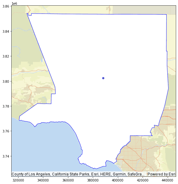
2. Use a specified distance and bin center to filter the bin geometries that are within the distance to the centroid of the California bins. Then use PySpark functions such as.describe() to generate basic summary statistics on the attribute columns of the bins nearby.

   Python

   Use dark colors for code blocksCopy

   1
   2
   3
   4
   5
   6
   7
   8
   9
   10
   11
   12
   13
   14
   15
   16
   17
   18
   19
   20
   21
   22
   23
   24
   25
   26
   27
   28
   29
   30
   31
   32
   33
   34
   35
   36
   37
   38
   39
   40
   41
   42
   43
   44
   45
   46
   47
   48
   49
   50
   51
   52
   53
   54
   55
   56
   57
   58
   59
   60
   61
   62
   63
   64
   65
   66
   67
   68
   69
   70
   71
   72
   73
   74
   75
   76
   77
   78
   79
   80
   81
   82
   83
   84
   85
   86
   87
   88
   89
   90
   91
   92
   93
   94
   95
   96
   97
   98
   99
   100
   101
   102
   103
   104
   105
   106
   107
   108
   109
   110
   111
   112
   113
   114
   115
   116
   117
   118
   119
   120
   121
   122
   123
   124
   125
   126
   127
   128
   129
   130
   131
   132
   133
   134
   135
   136
   137
   138
   139
   140
   141
   142
   143
   144
   145
   146
   147
   148
   149
   150
   151
   152
   153
   distance = 50000
   
   bin_center = la_pop_bin_center.select(ST.as_text("bin_center").alias("bin_center_text"))
   bin_center_str = [str(row["bin_center_text"]) for row in bin_center.collect()][0]
   
   geom_near = la_ozone \
           .withColumn("bin_center_text", F.lit(bin_center_str)) \
           .withColumn("bin_center", ST.point_from_text("bin_center_text")) \
           .withColumn("geom_near_center", ST.dwithin("bin_center", "point", distance)) \
           .where("geom_near_center == 'true'")
   
   geom_near.select("STATION","AV8TOP","MAXDAY","MONITOR").describe().show()
   
   Result

   Use dark colors for code blocksCopy

   1
   2
   3
   4
   5
   6
   7
   8
   9
   +-------+------------------+------------------+------------------+------------------+
   |summary|           STATION|            AV8TOP|            MAXDAY|           MONITOR|
   +-------+------------------+------------------+------------------+------------------+
   |  count|                11|                11|                11|                11|
   |   mean|128.54545454545453| 6.168621727272727|13.090909090909092| 70128.54545454546|
   | stddev|153.74222818494835|1.5321050204499749|2.9139164522870398|153.74222818494746|
   |    min|                60|          3.157258|                 8|             70060|
   |    max|               591|          8.241935|                18|             70591|
   +-------+------------------+------------------+------------------+------------------+

Visualize bins results

Visualizing bins results provides a quick representation of how your data is distributed spatially. You can visualize bins overlaid with geometry records to identify spatial patterns or attribute characteristics. You can also visualize with basemaps to put the bin results in geographical context.

1. Call st.plot on the DataFrame containing the bins column.

   Python

   Use dark colors for code blocksCopy

   1
   2
   3
   4
   5
   6
   7
   8
   9
   10
   11
   12
   13
   14
   15
   16
   17
   18
   19
   20
   21
   22
   23
   24
   25
   26
   27
   28
   29
   30
   31
   32
   33
   34
   35
   36
   37
   38
   39
   40
   41
   42
   43
   44
   45
   46
   47
   48
   49
   50
   51
   52
   53
   54
   55
   56
   57
   58
   59
   60
   61
   62
   63
   64
   65
   66
   67
   68
   69
   70
   71
   72
   73
   74
   75
   76
   77
   78
   79
   80
   81
   82
   83
   84
   85
   86
   87
   88
   89
   90
   91
   92
   93
   94
   95
   96
   97
   98
   99
   100
   101
   102
   103
   104
   105
   106
   107
   108
   109
   110
   111
   112
   113
   114
   115
   116
   117
   118
   119
   120
   121
   122
   123
   124
   125
   126
   127
   128
   129
   130
   131
   132
   133
   134
   135
   136
   137
   138
   139
   140
   141
   142
   143
   144
   145
   146
   147
   148
   149
   150
   151
   152
   153
   # Plot square bins of ozone point data
   bin_stats.st.plot(geometry="bin_geometry",facecolor="lightgrey", edgecolor="white", basemap="streets", figsize=(10, 10))
   
   

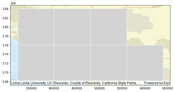
2. Overlay the point geometry with the bins to better visualize the spatial relationships.

   Python

   Use dark colors for code blocksCopy

   1
   2
   3
   4
   5
   6
   7
   8
   9
   10
   11
   12
   13
   14
   15
   16
   17
   18
   19
   20
   21
   22
   23
   24
   25
   26
   27
   28
   29
   30
   31
   32
   33
   34
   35
   36
   37
   38
   39
   40
   41
   42
   43
   44
   45
   46
   47
   48
   49
   50
   51
   52
   53
   54
   55
   56
   57
   58
   59
   60
   61
   62
   63
   64
   65
   66
   67
   68
   69
   70
   71
   72
   73
   74
   75
   76
   77
   78
   79
   80
   81
   82
   83
   84
   85
   86
   87
   88
   89
   90
   91
   92
   93
   94
   95
   96
   97
   98
   99
   100
   101
   102
   103
   104
   105
   106
   107
   108
   109
   110
   111
   112
   113
   114
   115
   116
   117
   118
   119
   120
   121
   122
   123
   124
   125
   126
   127
   128
   129
   130
   131
   132
   133
   134
   135
   136
   137
   138
   139
   140
   141
   142
   143
   144
   145
   146
   147
   148
   149
   150
   151
   152
   153
   # Plot Ozone station data overlay with bins
   bin_ax = bin_stats.st.plot(geometry="bin_geometry",facecolor="lightgrey", edgecolor="white", basemap="streets", figsize=(10, 10))
   ozone_points = la_ozone.st.plot(ax=bin_ax)
   
   

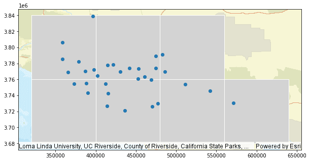
   To learn more about visualization, see the tutorial on visualizing results using st.plot().

3. Add a color ramp to the plotted bins to represent the count values.

   Python

   Use dark colors for code blocksCopy

   1
   2
   3
   4
   5
   6
   7
   8
   9
   10
   11
   12
   13
   14
   15
   16
   17
   18
   19
   20
   21
   22
   23
   24
   25
   26
   27
   28
   29
   30
   31
   32
   33
   34
   35
   36
   37
   38
   39
   40
   41
   42
   43
   44
   45
   46
   47
   48
   49
   50
   51
   52
   53
   54
   55
   56
   57
   58
   59
   60
   61
   62
   63
   64
   65
   66
   67
   68
   69
   70
   71
   72
   73
   74
   75
   76
   77
   78
   79
   80
   81
   82
   83
   84
   85
   86
   87
   88
   89
   90
   91
   92
   93
   94
   95
   96
   97
   98
   99
   100
   101
   102
   103
   104
   105
   106
   107
   108
   109
   110
   111
   112
   113
   114
   115
   116
   117
   118
   119
   120
   121
   122
   123
   124
   125
   126
   127
   128
   129
   130
   131
   132
   133
   134
   135
   136
   137
   138
   139
   140
   141
   142
   143
   144
   145
   146
   147
   148
   149
   150
   151
   152
   153
   bin_ax = bin_stats.st.plot(geometry="bin_geometry", cmap_values="count_station", cmap="Greys", edgecolor="black", basemap="streets", figsize=(10, 10))
   ozone_points = la_ozone.st.plot(ax=bin_ax, cmap='Reds', cmap_values="AV8TOP")
   
   

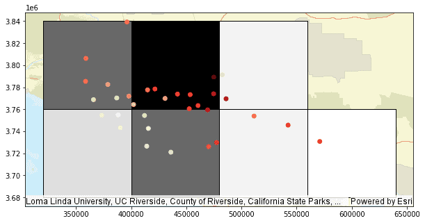
4. Close out the temp directories created at the beginning of the tutorial.

   Python

   Use dark colors for code blocksCopy

   1
   2
   3
   4
   5
   6
   7
   8
   9
   10
   11
   12
   13
   14
   15
   16
   17
   18
   19
   20
   21
   22
   23
   24
   25
   26
   27
   28
   29
   30
   31
   32
   33
   34
   35
   36
   37
   38
   39
   40
   41
   42
   43
   44
   45
   46
   47
   48
   49
   50
   51
   52
   53
   54
   55
   56
   57
   58
   59
   60
   61
   62
   63
   64
   65
   66
   67
   68
   69
   70
   71
   72
   73
   74
   75
   76
   77
   78
   79
   80
   81
   82
   83
   84
   85
   86
   87
   88
   89
   90
   91
   92
   93
   94
   95
   96
   97
   98
   99
   100
   101
   102
   103
   104
   105
   106
   107
   108
   109
   110
   111
   112
   113
   114
   115
   116
   117
   118
   119
   120
   121
   122
   123
   124
   125
   126
   127
   128
   129
   130
   131
   132
   133
   134
   135
   136
   137
   138
   139
   140
   141
   142
   143
   144
   145
   146
   147
   148
   149
   150
   151
   152
   153
   import shutil
   if os.path.exists(ca_data_path): shutil.rmtree(ca_data_path)
   if os.path.exists(ozone_data_path): shutil.rmtree(ozone_data_path)