Semantic segmentation
Semantic segmentation, also known as pixel-based classification, is an important task in which we classify each pixel of an image as belonging to a particular class. In GIS, segmentation can be used for land cover classification or for extracting roads or buildings from satellite imagery.
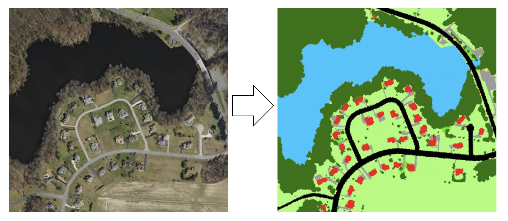
Figure 1. Semantic segmentation
The goal of semantic segmentation is the same as traditional image classification in remote sensing, which is usually conducted by applying traditional machine learning techniques such as random forest and maximum likelihood classifier. Like image classification, there are also two inputs for semantic segmentation.
- An raster image that contains serveral bands,
- A label image that contains the label for each pixel.
There are many semantic segmentation algorithms such as U-net, Mask R-CNN, Feature Pyramid Network (FPN), etc. In this guide, we will mainly focus on U-net which is one of the most well-recogonized image segmentation algorithms and many of the ideas are shared among other algorithms.
To follow the guide below, we assume that you have some basic understanding of the convolutional neural networks (CNN) concept. You can refresh your CNN knowledge by going through this short paper “A guide to convolution arithmetic for deep learning”.
U-net architecture
U-net was originally invented and first used for biomedical image segmentation. Its architecture can be broadly thought of as an encoder network followed by a decoder network. Unlike classification where the end result of the the deep network is the only important thing, semantic segmentation not only requires discrimination at pixel level but also a mechanism to project the discriminative features learnt at different stages of the encoder onto the pixel space.
-
The encoder is the first half in the architecture diagram (Figure 2). It usually is a pre-trained classification network like VGG/ResNet where you apply convolution blocks followed by a maxpool downsampling to encode the input image into feature representations at multiple different levels.
-
The decoder is the second half of the architecture. The goal is to semantically project the discriminative features (lower resolution) learnt by the encoder onto the pixel space (higher resolution) to get a dense classification. The decoder consists of upsampling and concatenation followed by regular convolution operations.
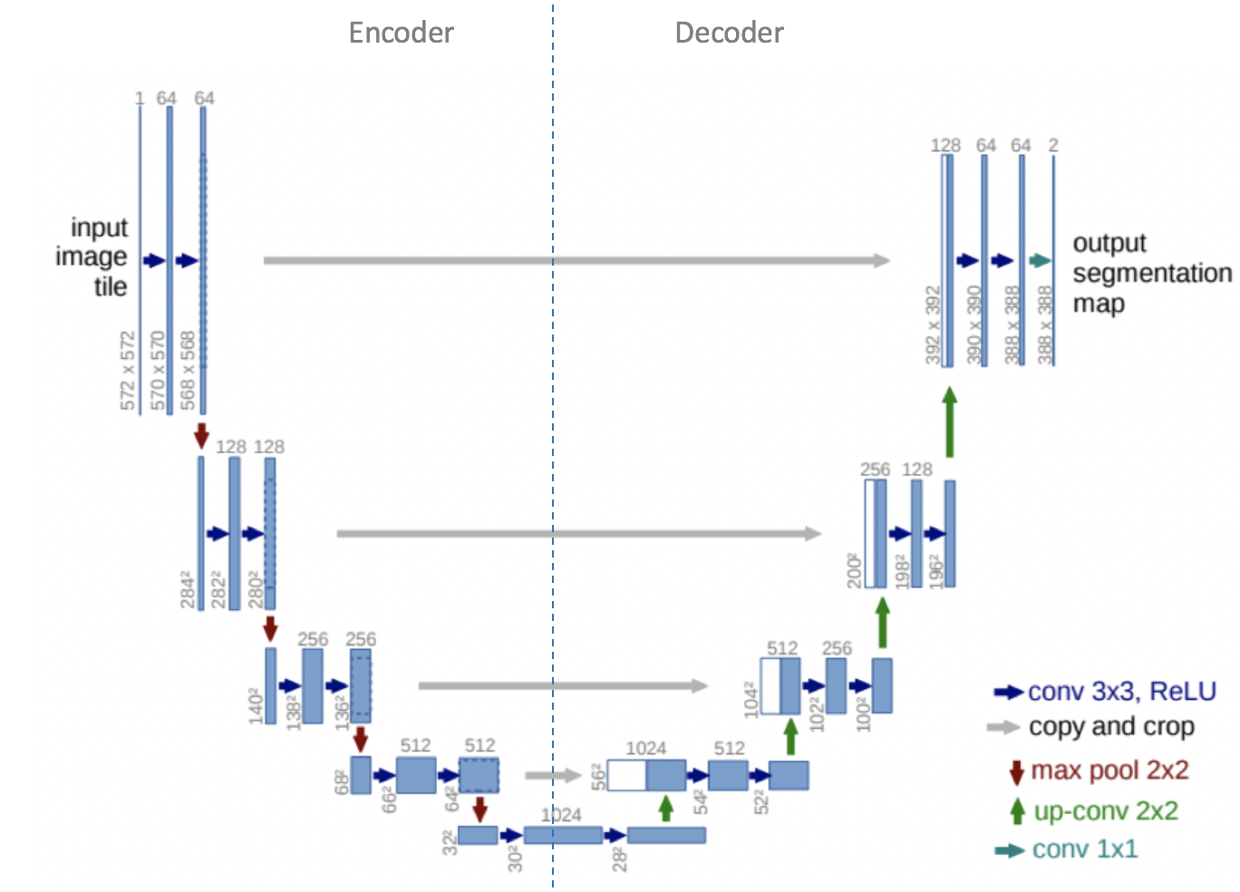
Figure 2. U-net architecture. Blue boxes represent multi-channel feature maps, while while boxes represent copied feature maps. The arrows of different colors represent different operations [1]
Upsampling in CNN might be new to those of you who are used to classification and object detection architecture, but the idea is fairly simple. The intuition is that we would like to restore the condensed feature map to the original size of the input image, therefore we expand the feature dimensions. Upsampling is also referred to as transposed convolution, upconvolution, or deconvolution. There are a few ways of upsampling such as Nearest Neighbor, Bilinear Interpolation, and Transposed Convolution from simplest to more complex. For more details, please refer to “A guide to convolution arithmetic for deep learning” we mentioned in the beginning.
Specifically, we would like to upsample it to meet the same size with the corresponding concatenation blocks from the left. You may see the gray and green arrows, where we concatenate two feature maps together. The main contribution of U-Net in this sense is that while upsampling in the network we are also concatenating the higher resolution feature maps from the encoder network with the upsampled features in order to better learn representations with following convolutions. Since upsampling is a sparse operation we need a good prior from earlier stages to better represent the localization.
In summary, unlike classification where the end result of the very deep network is the only important thing, semantic segmentation not only requires discrimination at pixel level but also a mechanism to project the discriminative features learnt at different stages of the encoder onto the pixel space.
U-net implementation in arcgis.learn
Armed with these fundamental concepts, we are now ready to define a U-net model. arcgis.learn allows us to define a U-net architecture just through a single line of code. For example:
unet = arcgis.learn.UnetClassifier(data, backbone=None, pretrained_path=None)
data is the returned data object from prepare_data function. backbone is used for creating the base of the UnetClassifier, which is resnet34 by default, while pretrained_path points to where pre-trained model is saved.
The UnetClassifier builds a dynamic U-Net from any backbone pretrained on ImageNet, automatically inferring the intermediate sizes. As you might have noticed, U-net has a lot fewer parameters than SSD, this is because all the parameters such as dropout are specified in the encoder and UnetClassifier creates the decoder part using the given encoder. You can tweak everything in the encoder and our U-net module creates decoder equivalent to that [2]. With that, the creation of Unetclassifier requires fewer parameters.
For more information about the API, please go to the API reference.
References
- [1] Olaf Ronneberger, Philipp Fischer, Thomas Brox: U-Net: Convolutional Networks for Biomedical Image Segmentation, 2015; arXiv:1505.04597.
- [2] Howard Jeremy. Fastai - Dynamic U-Net. https://www.youtube.com/watch?v=0frKXR-2PBY. Accessed 2 September 2019.