Introduction
The arcgis.learn module has an efficient point cloud classification model called PointCNN [1], which can be used to classify a large number of points in a point cloud dataset. In general, point cloud datasets are gathered using LiDAR sensors, which apply a laser beam to sample the earth's surface and generate high-precision x, y, and z points. These points, are known as 'point clouds' and are commonly generated through the use of terrestrial and airborne LiDAR.
Point clouds are collections of 3D points that carry the location, measured in x, y, and z coordinates. These points also have some additional information like 'GPS timestamps', 'intensity', and 'number of returns'. The intensity represents the returning strength from the laser pulse that scanned the area, and the number of returns shows how many times a given pulse returned. LiDAR data can also be fused with RGB (red, green, and blue) bands, derived from imagery taken simultaneously with the LiDAR survey.
Point cloud classification are based on the type of object that reflected the laser pulse. For example, a point that reflects off the ground is classified into the ground category. LiDAR points can be classified into different categories like buildings, trees, highways, water, etc. These different classes have numeric codes assigned to them. Point cloud data is typically stored in the industry-standard file format - LAS.

Figure 1. Visualization of point cloud dataset with RGB values
[3]. The features apart from x, y, and z values, such as intensity and number of returns are quite valuable for the task of classification, but at the same time, they are sensor-dependent and could become the main reasons for loss of generalization.
Point cloud classification is a task where each point in the point cloud is assigned a label, representing a real-world entity (see Figure 1). And similar to how it's done in traditional methods, for deep learning, the point cloud classification process involves training – where the neural network learns from an already classified (labeled) point cloud dataset, where each point has a unique class code. These class codes are used to represent the features that we want the neural network to recognize.

Figure 2. On the left side, raw LiDAR points can be seen. And for the same area, on the right side, we have classified points, where class codes are assigned to different colors
[2].
In deep learning workflows for point cloud classification, one should not use a ‘thinned-out’ representation of a point cloud dataset that preserves only class codes of interest but drops a majority of the undesired return points, as we would like the neural network to learn and be able to differentiate points of interest and those that are not. Likewise, additional attributes that are present in training datasets, for example, Intensity, RGB, number of returns, etc (see Figure 2). will improve the model’s accuracy but could inversely affect it if those parameters are not correct in the datasets that are used for inferencing.
It is in this aspect of point cloud classification where deep learning and neural networks provide an efficient and scalable architecture for classification of the input point cloud data, and with huge potential to render manual or semi assisted classification of point clouds obsolete. With this background let’s look at how the PointCNN model in arcgis.learn can be used for the classification of point cloud data.
Though the PointCNN network emulates traditional convolution neural networks and is a generalization of CNNs such as those that operate to extract features from imagery, it also introduces a novel approach to feature learning from point clouds – by accounting for the irregular and unordered nature of point clouds, which is not typically encountered when processing data represented in dense grids – for example in the case of images. This key ability of PointCNN, where it simultaneously weights and permutes the input features before applying a typical convolution on the transformed features, is known as X-Conv. Another feature of PointCNN that makes it appealing is its capability to consider the point shapes while being invariant to order - making it ideal for classification of point clouds, and in some cases even better suited than neural networks designed specifically for point clouds (such as PointNet++).
When training a PointCNN model, the raw point cloud dataset is first converted into blocks of points containing a specific number of points. These blocks then get passed into the model for training along with their labels. A similar process is followed when using the model for predictions as well.
PointCNN architecture
The PointCNN network for point cloud classification has a similar architecture to U-Net, as described in the How U-net works guide. Here too, we use an encoder-decoder paradigm, where the encoder reduces the number of points while increasing the number of channels. Then, the decoder part of the network increases the number of points, and the number of channels is incrementally reduced. The network also uses ‘skip connections’ like how it's done in the U-Net architecture.

Figure 3. A Generalized representation of a PointCNN for classification architecture
[1]. In each X-Conv operation, N represents the number of points in the next layer, C represents the number of channels, K represents the number of nearest neighbors and D represents the dilation rate
[1].
The difference is that the network processes a block of points as input and uses the X-Conv operation instead of Conv2D.
To state it succinctly, PointCNN differs from conventional grid-based CNNs primarily due to the application of X-Conv layers. Even then, the general process is like, how CNNs are used in grid-based convolution frameworks. The main differences are with respect to:
- The way the local regions are extracted, K ⇥K patches vs. K neighboring points around representative points (see Figure 3).
- The way the information from local regions is learned (Conv vs. X-Conv) [1].
X-Conv operation
As described in the Introduction section, a core part of the PointCNN framework is the X-Conv operation which is analogous to the convolution operation in CNNs. This operator performs a series of operations on a processed form of point cloud blocks, such as sampling and normalization using K-Nearest Neighbors.
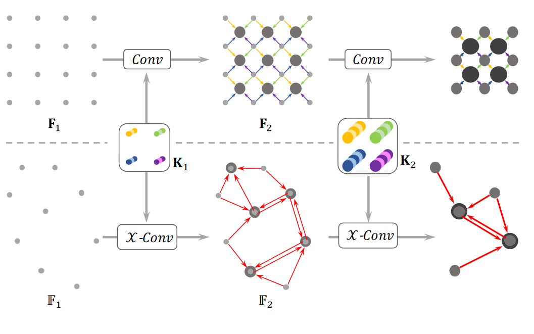
Figure 4. A diagram illustrating the differences and similarities of hierarchical convolution and PointCNN. The process above the dotted line denotes CNN in regular grids where convolutions are recursively applied on local grid patches. The process involves grid reductions – as done similarly in raster processing or meshing reducing the grid resolution successively (4X4⇥3X3⇥2X2), while increasing the channel number (visualized by dot thickness). Similarly, in point clouds, X-Conv is recursively applied to “project” or “aggregate” information, from the neighborhoods into fewer representative points (9⇥5⇥2) but each with richer information
[1].
Let's illustrate this step with an example. The first step involves sampling several points, let's call it sample P from the input set of points N. Then, for the P number of points, we find K nearest neighbors from N points (see Figure 4). This process is performed to form a local neighborhood of points for each point in P. This local neighborhood of points is then brought to a local coordinate space for each neighborhood. After these operations, we get an array of points of the shape (P, K, 3+E), where E is the number of extra features present (such as intensity, RGB values, or the number of returns), other than x, y, and z.
Implementation in arcgis.learn
When training a PointCNN model using arcgis.learn, the raw point cloud dataset in LAS files is first converted into blocks of points, containing a specific number of points along with their class codes.

Figure 5.
Prepare Point Cloud Training Datatool in ArcGIS Pro.
For this step of exporting the data into an intermediate format, use Prepare Point Cloud Training Data tool, in the 3D Analyst extension (see Figure 5).
These exported blocks are used to create a data bunch object that is passed into the PointCNN model for training.
output_path=r'C:/project/training_data.pctd'
data = prepare_data(output_path, dataset_type='PointCloud', batch_size=2)
pointcnn = PointCNN(data)
pointcnn.fit(20)
After training the PointCNN model, compute_precision_recall() method can be used to compute, per-class metrics (precision, recall, and f1-score) with respect to validation data. And save() method can be used to save the model.
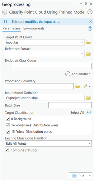
Figure 6.
Classify Points Using Trained Modeltool.
For inferencing, use Classify Points Using Trained Model tool, in the 3D Analyst extension (see Figure 6).
Main features available during the inferencing step:
-
Target classification: selective classification for flexibility and control in trained model's predictions.
-
Preserving specific classes in input data from modification: this can be used for updating old datasets and for noise control in model's prediction.
Detailed tool references and resources for point cloud classification using deep learning in ArcGIS Pro can be found here.
For advanced users
We can also specify all the additional parameters while initializing PointCNN by using certain keyword arguments. One of those is encoder_params keyword argument, which can be used to specify the number of output channels for each layer in the encoder. The decoder of the network is built accordingly.
There are mainly four things that we need to define in the encoder: out_channels, P, K, and D. All of these are supplied as a 'python list'. The out_channel specifies the number of channels after each layer. While, for each layer P, K and D specify the 'number of points', 'k-nearest-neighbor', and 'dilation rate' respectively. Additionally, one can specify m, which is the multiplicative factor, that is multiplied by each element of the out_channel list. The other keyword arguments are dropout and sample_point_num. The dropout keyword argument specifies the amount of regularization we want to add to the model, with its value ranging between 0 and 1. The sample_point_num keyword argument specifies the number of points that will actually be used for training the model. It is usually equal to the number of maximum points in a block while exporting the point cloud dataset.
A typical usage looks like:
pointcnn = PointCNN(data=data,
                    encoder_params={'out_channels':[16, 32, 64, 96],
                                    'P':[-1, 768, 384, 128],
                                    'K':[12, 16, 16, 16],
                                    'D':[1, 1, 2, 2],
                                    'm':8
                                    },
                    dropout=0.5,
                    sample_point_num=8192
                   )
Best practices for PointCNN workflow
The following tips and best-practices can be used while using PointCNN:
- The 3D deep learning tools in the 3D Analyst extension, takes care of the coordinate system, and related discrepancies, automatically. So, one can train a model using ArcGIS Pro on a dataset with a metric coordinate system, then use that trained model on a dataset with any other coordinate system, and vice-versa without any need for re-projection.
- High-quality labeled data will result in a better-trained model. For generalization and robustness of the trained model, significant diversity or variety should be present in the training data, in terms of geography, building architectures, terrains, object-related variations, etc.
- If the object of interest is significantly larger or smaller in size than the default value of
Block Size, then a better value can be used for improving the results further. Like, for a dataset in a metric coordinate system, a 'warehouse' won't fit in a '50 meter' x '50 meter'Block Size, hence theBlock Sizecan be increased in this case.
- Through a series of experiments, it was found that an additional one or two
extra_featuresapart from X, Y, and Z usually works best, in most cases. Over usage of 'extra attributes' for model training might reduce generalization, i.e. 'how generic the trained model will be'.
- Deciding which 'extra attributes' to consider, depends upon the properties of the object of interest, the nature of noise, sensor-specific attributes, etc.
- It is recommended to filter or withheld points that belong to the 'high noise' class from the dataset.
- If the training and validation dataset is very large and each epoch is taking a lot of time to complete, then
iters_per_epochcan be used to see the epoch/training table quickly by reducing the time taken for the completion of an epoch. This is achieved by a random selection/filtering of fewer batches, governed by the user-provided value ofiters_per_epoch. So in each epoch, the model is exposed to a lesser number of randomly selected batches, this results in faster completion of an epoch, but it can lead to more numbers of epochs before the model converges.
mask_classfunctionality inshow_results()can be used for analyzing any inter-class noises present in the validation output. This can be used to understand which classes need more diversity in training data or need an increase in its number of labeled points (See Figure 7).

Figure 7. Class-based masking of points, to understand the nature of noise in the prediction.
- The default value of
max_display_pointinshow_batch()andshow_results()is set to '20000', keeping the rendering-related browser limitation in mind, which can occur for very dense point clouds. This value can be increased if needed, for detailed visualization, within the browser itself.
Target ClassificationandClass Preservationin Classify Points Using Trained Model tool, can be used in conjunction to combine the knowledge of multiple trained models for a single scene.
- Parameters like,
classes_of_interestandmin_pointsare especially useful when training a model for SfM or mobile/terrestrial point clouds. In specific scenarios when the 'training data' is not small, these features can be very useful in speeding up the 'training time', improving the convergence during training, and addressing the class imbalance up to some extent.
- Fine-tuning a pretrained model is only preferred if the 'object of interest' is either same or similar, else it is not beneficial. Otherwise, fine-tuning a pretrained model can save cost, time, and compute resources while providing better accuracy/quality in results.
- Class codes can be given a meaningful name, using
class_mapping. The names of the class codes are saved inside the model, which is automatically retrieved by Classify Points Using Trained Model tool and Train Point Cloud Classification Model tool, when a trained model is loaded.
- For fine-tuning a model with default architecture settings; 'Class Structure', 'Extra Attributes', and 'Block Point Limit' should match between the pretrained model and the exported 'training data'.
References
[1] Li, Y., Bu, R., Sun, M., Wu, W., Di, X., & Chen, B. (2018). PointCNN: Convolution On
[2] Dmitry Kudinov. (2019). PointCNN: replacing 50,000 man hours with AI.
https://medium.com/geoai/pointcnn-replacing-50-000-man-hours-with-ai-d7397c1e7ffe
[3] AutoDesk. (2020). About Point Cloud Color Stylization and Visual Effects.
https://knowledge.autodesk.com/support/autocad/learn-explore/caas/CloudHelp/cloudhelp/2020/ENU/AutoCAD-Core/files/GUID-75EBFA48-CB7E-4E91-A1BB-167D96A7119F-htm.html