The features module packs a set of data summarization tools to calculate total counts, lengths, areas, and basic descriptive statistics of features and their attributes within areas or near other features. You can access these tools using the summarize_data sub module.
Aggregate points
In this example, let us observe how to use aggregate_points tool to summarize data from spot measurements by area. To learn more about this tool and the formula it uses, refer to the documentation here.
# connect to GIS
from arcgis.gis import GIS
gis = GIS("portal url", "username", "password")
eq_search = gis.content.search(query="title:World Earthquake Locations owner:api_data_owner", item_type="Feature Layer Collection", max_items=1)
eq_item = eq_search[0]
eq_item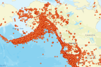
# search for USA states - area / polygon data
states_search = gis.content.search("title:'USA States (Generalized)'",
                                   "feature layer", max_items=-1)
states_item = states_search[0]
states_item
Let's draw the layers on a map and observe how they are distributed.
map1 = gis.map("USA")
map1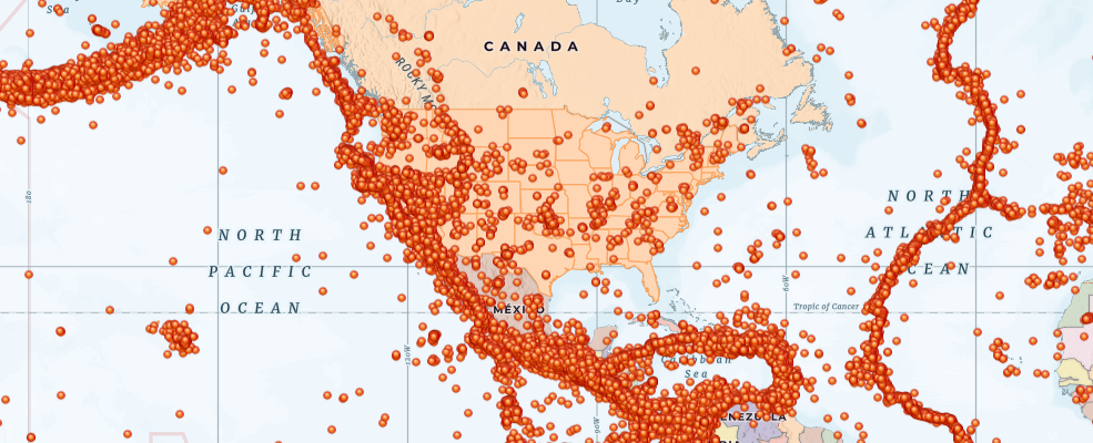
map1.center = [36, -98]
map1.zoom = 3map1.content.add(states_item)map1.content.add(eq_item)Aggregate earthquakes by state
As you can see, a number of earthquakes fall on the boundary of tectonic plates (ring of fire). However, there are a few more dispersed into other states. It would be interesting to aggregate all the earthquakes by state and plot that as a chart.
The aggregate_points tool in the summarize_data sub module is a valid candidate for such analyses. The example below shows how to run this tool using ArcGIS API for Python.
To start with, let us access the layers in the states and earthquakes items and view their attribute information to understand how the data can be summarized.
eq_fl = eq_item.layers[0]
states_fl = states_item.layers[0]
We have accessed the layers in the items as FeatureLayer objects. We can query the fields property to understand what kind of attribute data is stored in the layers.
#query the fields in eq_fl layer
for field in eq_fl.properties.fields:
    print(field['name'])
Event_Id Community_Decimal_Intensity Event_Detail Distance_from_Epicenter__degree Felt_Reports Azimuthal_Gap__degrees_ Event_Magnitude Magnitude_Type Shake_Intensity Source_Network Seismic_Stations Location_Name Residual_Travel_Time__seconds_ Event_Significance Network_Sources Review_Status Event_Time Event_Title Tsunami_Warning Event_Type Product_Types Last_Updated Event_Page Latitude Longitude Elevation__meters_ Depth__kilometers_ OBJECTID Event_Time_1 Event_Type_1 ObjectId2
field_names = [f["name"] for f in states_fl.properties.fields]for a,b,c,d,e in zip(field_names[0::10], field_names[1::10], field_names[2::10], field_names[3::10], field_names[4::10]):
print(f"{a:17}{b:17}{c:17}{d:17}{e:17}")
print(f"{field_names[56]:17}{field_names[57]:17}")FID STATE_NAME STATE_FIPS SUB_REGION STATE_ABBR BLACK AMERI_ES ASIAN HAWN_PI HISPANIC AGE_5_9 AGE_10_14 AGE_15_19 AGE_20_24 AGE_25_34 AGE_85_UP MED_AGE MED_AGE_M MED_AGE_F HOUSEHOLDS MHH_CHILD FHH_CHILD FAMILIES AVE_FAM_SZ HSE_UNITS CROP_ACR12 AVE_SALE12 SQMI Shape__Area Shape__Length Shape__Area_2 Shape__Length_2
Let us aggreate the points by state and summarize the magnitude field and use mean as the summary type.
# this cell will take a few minutes to execute because of several data points
from arcgis.features import summarize_data
sum_fields = ['Event_Magnitude Mean', 'Depth__kilometers_ Min']
eq_summary = summarize_data.aggregate_points(point_layer = eq_fl,
                                            polygon_layer = states_fl,
                                            keep_boundaries_with_no_points=False,
                                            summary_fields=sum_fields)
{"cost": 478.947}
When running the tool above, we did not specify a name for the output_name parameter. Consequently, the analyses results were not stored on the portal, and instead stored in the variable eq_summary.
eq_summary{'aggregated_layer': <FeatureCollection>, 'group_summary': ''}# access the aggregation feature colleciton
eq_aggregate_fc = eq_summary['aggregated_layer']
#query this feature collection to get a data as a feature set
eq_aggregate_fset = eq_aggregate_fc.query()FeatureSet objects support visualizing attribute information as a pandas dataframe. This is a neat feature since you do not have to iterate through each feature to view their attribute information.
Let us view the summary results as a pandas dataframe table. Note, the aggregate_points tool appends the polygon layer's original set of fields to the analysis result in order to provide context.
aggregation_df = eq_aggregate_fset.sdf
aggregation_df.head()| OBJECTID | STATE_NAME | STATE_FIPS | SUB_REGION | STATE_ABBR | POPULATION | POP_SQMI | POP2010 | POP10_SQMI | WHITE | ... | GlobalID | Shape__Area_2 | Shape__Length_2 | Shape_Length | Shape_Area | mean_Event_Magnitude | min_Depth__kilometers_ | Point_Count | AnalysisArea | SHAPE | |
|---|---|---|---|---|---|---|---|---|---|---|---|---|---|---|---|---|---|---|---|---|---|
| 0 | 1 | Wyoming | 56 | Mountain | WY | 598332 | 6.1 | 563626 | 5.8 | 511279 | ... | {9DC7C7AC-FE50-46FF-A98A-BC9B99E0CED0} | 474117105945.773438 | 2775149.430913 | 2775149.430947 | 474117105972.575684 | 4.550545 | -1.4 | 110 | 253293.67329 | {"rings": [[[-11583195.4614, 5115880.653200000... |
| 1 | 3 | Alaska | 02 | Pacific | AK | 744733 | 1.3 | 710231 | 1.2 | 473576 | ... | {FC1D546E-050D-40E0-8674-D380F839AD76} | 8101401247192.390625 | 59249543.508505 | 59249543.507812 | 8101401247161.800781 | 4.474101 | -3.0 | 2802 | 1493247.177689 | {"rings": [[[-17959594.8053, 8122953.575199999... |
| 2 | 5 | North Dakota | 38 | West North Central | ND | 793399 | 11.2 | 672591 | 9.5 | 605449 | ... | {4C973C13-C535-45DD-B5CB-0BD837DAE90D} | 400989888326.039062 | 2688189.824234 | 2688189.824286 | 400989888305.082947 | 5.5 | 0.0 | 1 | 183403.48984 | {"rings": [[[-10990621.962, 5770462.616400003]... |
| 3 | 6 | South Dakota | 46 | West North Central | SD | 880051 | 11.4 | 814180 | 10.6 | 699392 | ... | {2064228A-2CC4-4E74-B492-34EF98939518} | 392302335744.371094 | 2824245.235541 | 2824245.23589 | 392302335746.93811 | 4.3 | 0.0 | 8 | 199912.09036 | {"rings": [[[-11442350.6328, 5311257.036700003... |
| 4 | 7 | Delaware | 10 | South Atlantic | DE | 971403 | 491.7 | 897934 | 454.5 | 618617 | ... | {C83CE019-1814-4B07-8111-6B414909808F} | 8823228994.324219 | 535395.672895 | 535395.672768 | 8823228992.748075 | 4.1 | 9.87 | 1 | 5321.669252 | {"rings": [[[-8427672.8732, 4658497.009999998]... |
5 rows × 63 columns
Let's narrow down the output fields to view the output fields from the summarize_data() operation.
aggregation_df[["STATE_NAME","SUB_REGION","STATE_ABBR","POP2010","POP10_SQMI","mean_Event_Magnitude","min_Depth__kilometers_"]].head()| STATE_NAME | SUB_REGION | STATE_ABBR | POP2010 | POP10_SQMI | mean_Event_Magnitude | min_Depth__kilometers_ | |
|---|---|---|---|---|---|---|---|
| 0 | Wyoming | Mountain | WY | 563626 | 5.8 | 4.550545 | -1.4 |
| 1 | Alaska | Pacific | AK | 710231 | 1.2 | 4.474101 | -3.0 |
| 2 | North Dakota | West North Central | ND | 672591 | 9.5 | 5.5 | 0.0 |
| 3 | South Dakota | West North Central | SD | 814180 | 10.6 | 4.3 | 0.0 |
| 4 | Delaware | South Atlantic | DE | 897934 | 454.5 | 4.1 | 9.87 |
Let's narrow this data down further to only those states that have had more than 25 earthquakes over the span of this data (1900 - 2023).
agg_gt25_df = aggregation_df.loc[aggregation_df["Point_Count"] > 25]len(agg_gt25_df)15
As we can see, over the time span of this data, only 15 of the 50 US States have had more than 25 earthquakes. Let us plot a bar chart to view which states had the most earthquakes.
%matplotlib inline
agg_gt25_df.plot('STATE_NAME','Point_Count', kind='bar')
<Axes: xlabel='STATE_NAME'>
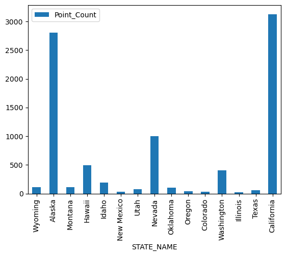
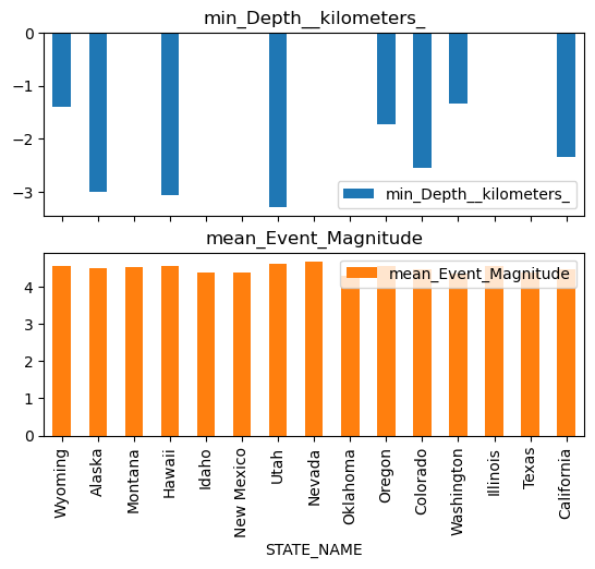
California and Alaska clearly top the list with the most earthquakes. Let us view what the average intensity and minimum depth is in the plots below:
agg_gt25_df.plot('STATE_NAME',['min_Depth__kilometers_', 'mean_Event_Magnitude'],kind='bar', subplots=True)array([<Axes: title={'center': 'min_Depth__kilometers_'}, xlabel='STATE_NAME'>,
<Axes: title={'center': 'mean_Event_Magnitude'}, xlabel='STATE_NAME'>],
dtype=object)