- 🔬 Data Science
- 🥠 Deep Learning and Instance Segmentation
Introduction
The workflow traditionally used to reconstruct 3D building models from aerial LiDAR is relatively straight-forward: the LiDAR point-cloud is transformed into a Digital Surface Model (DSM) raster, then inspected by human editors for buildings present. If a building is found, one or more polygons describing the roof form of the building is manually digitized, e.g. if it is a large hip roof with two gable outlets, there will be three polygons (one hip and two gables on top) drawn by the editor. Once all the roofs are described that way, a set of ArcGIS Procedural rules is applied to extrude the building models using the manually digitized roof segments, with heights and ridge directions computed from the DSM.

Figure 1. 3D building reconstruction from Lidar example: a building with complex roof shape and its representation in visible spectrum (RGB), Aerial LiDAR, and corresponding roof segments digitized by a human editor. The last one is a 3D reconstruction of the same building using manually digitized masks and ArcGIS Procedural rules.
The most time-consuming and expensive step in the above workflow is the manual search and digitization of the roof segment polygons from a DSM raster. In this notebook, we are going to focus on this challenging step and demonstrate how to detect instances of roof segments of various types using instance segmentation to make the process more efficient. The workflow consists of four major steps: (1) extract training data, (2) train a deep learning instance segmentation model, (3) model deployment and roof segments detection and (4) 3D enabling the detected segments.
Prerequisites
Complete data required to run this sample is packaged together in a project package and can be downloaded from here. You are also required to download the rule package used in Part 4 of this notebook from here.
Below are the items present in the project package shared:
- D1_D2_D3_Buildings_1: labelled feature data for training data preparation
- R7_nDSM_TestVal: raster image for training data preparation
- DSM_AOI_Clip: DSM raster for area of interest, required during model inferencing
- DTM_AOI_Clip: DTM raster for area of interest, required during model inferencing
- DSM_AOI_Clip_DetectObjects_26032020_t4_220e: sample results obtained from the trained MaskRCNN model inferenced on area of interest obtained after performing part 3 of the notebook
- DSM_AOI_Clip_DetectObjects_26032020_t4_220e_selection_3dEnabling: sample 3D enabled roof segments obtained after performing part 4 of the notebook
Moreover, there is a toolbox (3d_workflow.tbx) in the 'Toolboxes' section of the project having the script (3dEnabling) to perform part 4 of the notebook.
Part 1 - Data Preparation
We started with two input data:
- A single-band raster layer (R7_nDSM_TestVal) with 2.25 square feet per pixel resolution converted from LiDAR point cloud (using the “LAS Dataset to Raster” geoprocessing tool)
- A feature class (D1_D2_D3_Buildings_1) that defines the location and label (i.e. flat, gable, hip, shed, mansard, vault, dome) of each roof segment.
We are using single band Lidar data which is essentially elevation to train our deep learning MaskRCNN model.

Figure 2. Example of different roof types (flat not shown).
Export training data
Export training data using 'Export Training data for deep learning' tool, detailed documentation here.
Input Raster: R7_nDSM_TestValOutput Folder: Set a location where you want to export the training data, it can be an existing folder or the tool will create that for you.Input Feature Class Or Classified Raster: D1_D2_D3_Buldings_1Image Format: TIFF formatTile Size X&Tile Size Ycan be set to 256Stride X&Stride Y: 128Meta Data Format: Select 'RCNN Masks' as the data format because we are training a MaskRCNN model.- In
Environmentstab set an optimumCell Size. For this example, as we have to perform the analysis on the LiDAR imagery, we used 0.2 cell size.

Figure 3. Export Training data screenshot from ArcGIS Pro.
arcpy.ia.ExportTrainingDataForDeepLearning(in_raster="R7_nDSM_TestVal",
out_folder=r"\Documents\PCNN\Only_nDSM",
in_class_data="D1_D2_D3_Buildings_1",
image_chip_format="TIFF",
tile_size_x=256,
tile_size_y=256,
stride_x=128,
stride_y=128,
output_nofeature_tiles="ONLY_TILES_WITH_FEATURES",
metadata_format="RCNN_Masks",
start_index=0,
class_value_field="None",
buffer_radius=0,
in_mask_polygons=None,
rotation_angle=0,
reference_system="MAP_SPACE",
processing_mode="PROCESS_AS_MOSAICKED_IMAGE",
blacken_around_feature="NO_BLACKEN",
crop_mode="FIXED_SIZE")
After filling all details and running the Export Training Data For Deep Learning tool, a code like above will be generated and executed. That will create all the necessary files needed for the next step in the 'Output Folder', and we will now call it our training data.
Part 2 - Model Training
You should already have the training chips with you exported from ArcGIS pro. Please change the path to your own export training data folder that contains "images" and "labels" folder. Note that we set a relatively small batch_size here on purpose as instance segmentation is a more computationally intensive task compared with object detection and pixel-based classification. If you run into "insufficient memory" issue during training, you can come back to adjust it to meet your own needs.
Necessary Imports
import os
from pathlib import Path

from arcgis.learn import prepare_data, MaskRCNN
#connect to GIS
from arcgis.gis import GIS
gis = GIS('home')Prepare data
We will now use the prepare_data() function to apply various types of transformations and augmentations on the training data. These augmentations enable us to train a better model with limited data and also prevent the model from overfitting. prepare_data() takes 3 parameters.
path: path of the folder containing training data.batch_size: No of images your model will train on each step inside an epoch, it directly depends on the memory of your graphic card. 8 worked for us on a 11GB GPU.imagery_type: It is a mandatory input to enable a model for multispectral data processing. It can be "landsat8", "sentinel2", "naip", "ms" or "multispectral".
training_data = gis.content.get('807425fa74f34d7695ec024eb934456c')
training_data
filepath = training_data.download(file_name=training_data.name)import zipfile
with zipfile.ZipFile(filepath, 'r') as zip_ref:
zip_ref.extractall(Path(filepath).parent)data_path = Path(os.path.join(os.path.splitext(filepath)[0]))data = prepare_data(data_path, batch_size=8, imagery_type='ms')Visualize a few samples from your training data
To get a sense of what the training data looks like, arcgis.learn.show_batch() method randomly picks a few training chips and visualizes them. Note that the masks representing different roof segments are overlaid upon the original images with red and pink colors.
rows: No of rows we want to see the results for.
data.show_batch(rows=2)
Load model architecture
Here we use Mask R-CNN [1], a well-recognized instance algorithm, to detect roof segments (Figure 3). A Mask R-CNN model architecture and a pretrained model has already been predefined in arcgis.learn, so we can just define it with a single line. Please refer to the guide on our developers' site for more information.
The idea of Mask R-CNN is to detect objects in an image while simultaneously generating a high-quality segmentation mask for each instance. In other words, it is like a combination of UNet and SSD and does two jobs in one go. This is also why it is relatively computationally more intensive.
model = MaskRCNN(data)
Figure 4. Mask R-CNN framework for instance segmentation [1]
Find an optimal learning rate
Learning rate is one of the most important hyperparameters in model training. arcgis.learn leverages fast.ai’s learning rate finder to find an optimum learning rate for training models. We can use the lr_find() method to find the optimum learning rate at which we can train a robust model fast enough.
# The users can visualize the learning rate of the model with comparative loss.
lr = model.lr_find()
lr
4.365158322401661e-05
Fit the model
Let's train it for a few epochs with the learning rate we have found. For the sake of time, we can start with 10 epochs.
model.fit(epochs=10, lr=lr)| epoch | train_loss | valid_loss | time |
|---|---|---|---|
| 0 | 2.769909 | 2.669544 | 06:09 |
| 1 | 2.142615 | 2.117454 | 06:38 |
| 2 | 1.951803 | 1.997903 | 07:03 |
| 3 | 1.843830 | 1.804779 | 07:50 |
| 4 | 1.687831 | 1.723288 | 08:12 |
| 5 | 1.534998 | 1.688702 | 07:52 |
| 6 | 1.503451 | 1.559698 | 07:48 |
| 7 | 1.417018 | 1.515242 | 07:40 |
| 8 | 1.335621 | 1.512897 | 07:36 |
| 9 | 1.238250 | 1.535544 | 07:26 |
Note that the validation loss actually goes higher, but this doesn't necessarily mean the result is getting bad. Because our training data is also missing many buildings, the loss sometimes tells the actual model performance, so let's look at the actual results instead.
Save the model
We will save the model which we trained as a 'Deep Learning Package' ('.dlpk' format). Deep Learning package is the standard format used to deploy deep learning models on the ArcGIS platform.
We will use the save() method to save the trained model. By default it will be saved to the 'models' sub-folder within our training data folder.
model.save('10e')Visualize results in validation set
Now we have the model, let's look at how the model performs. There are 3 modes when visualizing the results.
bbox- For visualizing only bounding boxes.mask- For visualizing only maskbbox_mask- For visualizing both mask and bounding boxes.
model.show_results(mode='bbox_mask', rows=2)
As we can see, with only 10 epochs, we are already seeing good results. We have trained it further till 220 epochs and were able to get promising results. Below are the results that we got from our model trained for 220 epochs.
Load a saved model to visualize results
To visualize results from a saved model, we can load it using load() function.
model.load('220e')model.show_results(mode='bbox_mask', rows=5, box_threshold=0.5)
Part 3 - Deploy Model and Detect Roof Segments
We will use saved model to detect objects using 'Detect Objects Using Deep Learning' tool available in both ArcGIS Pro and ArcGIS Enterprise. For this sample, we will use the DSM image for our area of Interest. You will find this image in the ArcGIS project you have downloaded with the name - DSM_AOI_Clip.
Input Raster: DSM_AOI_ClipOutput Detect Objects: DSM_AOI_Clip_DetectObjectsModel Definition: path to the model emd filepadding: The 'Input Raster' is tiled and the deep learning model runs on each individual tile separately before producing the final 'detected objects feature class'. This may lead to unwanted artifacts along the edges of each tile as the model has little context to detect objects accurately. Padding as the name suggests allows us to supply some extra information along the tile edges, this helps the model to predict better.batch_size: 4threshold:0.4return_bboxes: FalseCell Size: Should be close to at which we trained the model, we specified that at the Export Training Data step .

Figure 5. Detect objects using Deep Learning screenshot from ArcGIS Pro
arcpy.ia.DetectObjectsUsingDeepLearning(in_raster="DSM_AOI_Clip",
out_detected_objects=r"sample.gdb\DSM_AOI_Clip_DetectObjects",
in_model_definition=r"\models\200e\200e.emd",
model_arguments="padding 56;batch_size 4;threshold 0.4;return_bboxes False;",
run_nms="NO_NMS",
confidence_score_field="Confidence",
class_value_field="Class",
max_overlap_ratio=0,
processing_mode = "PROCESS_AS_MOSAICKED_IMAGE")

Figure 6. A subset of detected different types of building roof forms (shown in different color)
Part 4 - 3D enabling the MaskRCNN results
The next step is to extrude object detection results in 3D using traditional Geoprocessing tools and Procedural rules. First, we used the “Regularize Building Footprint” tool from the 3D Analyst toolbox to regularize raw detections. Next, we used surface elevation and DSM rasters to acquire the base elevation for each building segment, and calculate the roof ridge direction. The final step was calling the “Features from CityEngine Rules” GP tool which applied a procedural rule to these polygons to achieve a final reconstruction of the 3D buildings.
All the pre-processing steps are recorded in a python script and shared with you in the form of a toolbox within your project. Double click on the script (3dEnabling).

Figure 7. Screenshot of location of the script to perform 3D enabling task
The 3dEnabling script takes the following inputs:
Input Masks: detected buildings from MaskRCNN model.DTM: 'DTM_AOI_Clip' image from the project.DSM: 'DSM_AOI_Clip' image from the project.Rule Package: 'LGIM_RFE_LOD2.rpk' rule package file from the project.Output Buildings: 3dEnabledPolygonsCell Size: Should be close to at which we trained the model, we specified that at the Export Training Data step.

Figure 8. 3dEnabling tool screenshot from ArcGIS Pro
arcpy.3dworkflow.3dEnabling(Input_Masks="DSM_AOI_Clip_DetectObjects",
DTM="DTM_AOI_Clip",
DSM="DSM_AOI_Clip",
Rule_Package=r"\Reconstruction_part2\LGIM_RFE_LOD2.rpk",
Output_Buildings=r"\reconstruction_part2.gdb\DSM_AOI_Clip_DetectObjects_3dEnabling")```
This tool converts the detection obtained from MaskRCNN model in 3D based on the rules defined in the rule package.
scene_item = gis.content.get('9ce6cf3170334c61bf3da25dacbdf553')from arcgis.map import Scene
scene1 = Scene(item = scene_item)
scene1.extent = {'spatialReference': {'latestWkid': 3857, 'wkid': 102100},
'xmin': -8919494.611200048,
'ymin': 2981619.558592063,
'xmax': -8918883.485987043,
'ymax': 2981867.4795709597}
scene1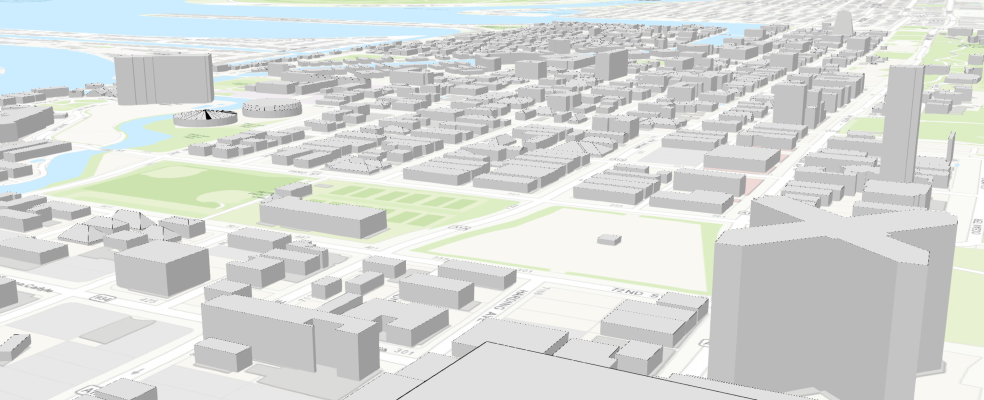
Here is a web map to showcase the results obtained from the notebook.
Conclusion
In this notebook, we have covered a lot of ground. In part 1, we discussed how to prepare and export training data from aerial Lidar data. In part 2, we demonstrated how to prepare the input data, train an instance segmentation model, visualize the results, as well as apply the model to an unseen image using the deep learning module in ArcGIS API for Python. In part 4, we discussed how the MaskRCNN results obtained can be converted in 3D using the toolbox shared.
References
[1] He, K., Gkioxari, G., Dollár, P. and Girshick, R., 2017. Mask r-cnn. In Proceedings of the IEEE international conference on computer vision (pp. 2961-2969).