- 🔬 Data Science
- 🥠 Deep Learning
- 🌍 GIS
- ☁️ Point Cloud Classification

Introduction
Classification of point clouds has always been a challenging task, due to its naturally unordered data structure. The workflow described in this sample is about going from raw unclassified point clouds to digital twins: near-perfect representation of real-world entities. Within the scope of this sample, we are only interested in 'digital twins of buildings' (3D building multipatches/models). This work can also be used for guidance, in other relevant use-cases for various objects of interest.
First, deep learning capabilities in 'ArcGIS API for Python' are utilized for point cloud classification, then 'ArcGIS Pro' and 'City Engine' are used for the GIS-related post-processing.
Further details on the PointCNN implementation in the API (working principle, architecture, best practices, etc.), can be found in the PointCNN guide, along with instructions on how to set up the Python environment. Additional sample notebooks related to PointCNN can be found in the sample notebook section on the website.
Before proceeding through this notebook, it is advised that you go through the API reference for PointCNN (prepare_data(), Transform3d(), and PointCNN()), along with the resources and tool references for point cloud classification using deep learning in ArcGIS Pro, found here.
Objectives:
- Classify building points using API's PointCNN model, where we train it for two classes: viz. 'Buildings' and 'Background'.
- Generate 3D building multipatches, from classified building points using 'ArcGIS Pro' and 'City Engine'.
Area of interest and pre-processing
Any airborne point cloud dataset and area of interest can be used. But for this sample, AHN3 dataset, provided by the Government of The Netherlands is considered [1], which is one of the highest quality open datasets available currently, in terms of accurate labels and point density. While the area of interest for this work is 'Amsterdam' and its nearby regions. Its unique terrain with canals and from modern to 17th - century architecture style makes it a good candidate for a sample.
Pre-processing steps:
-
Uncompress, the downloaded AHN3 dataset's
.lazfiles, into.lasformat. (Refer, ArcGIS Pro's Convert LAS tool.) -
Reassign class codes, so that only two classes remain in the data: ‘Buildings’ and ‘Background’ (Refer, ArcGIS Pro's Change LAS Class Codes tool). In this sample, ASPRS-defined class codes are followed (optional, for the PointCNN workflow). Hence, '6' is used to represent 'Buildings'. And reserved-class code '19' is used to represent 'Background' (rest of the points), as it is also a class which the model will learn about, along with 'Buildings' class. So, the class code for 'points in undefined state': '1' and ' points in never-classified state': '0', are not used to represent 'Background' class.
-
Split the
.lasfiles into three unique sets, one for training, one for validation, and one for testing. Create LAS datasets for all three sets using the 'Create LAS Dataset' tool. There is no fixed rule, but generally, the validation data for point clouds in.lasformat should be at least 5-10 % (by size) of the total data available, with appropriate diversity within the validation dataset. (For ease in splitting the big.lasfiles into the appropriate ratios, ArcGIS Pro's 'Tile LAS' tool can be used.) -
Alternatively, polygons can also be used to define regions of interest that should be considered as training or validation datasets. These polygons can be used later in the export tool. If the dataset is very large, then the 'Build LAS Dataset Pyramid' tool can be leveraged for faster rendering/visualization of the data, which will also help in exploring and splitting the dataset.
Data preparation
Imports:
from arcgis.learn import prepare_data, Transform3d, PointCNN
from arcgis.gis import GIS
gis = GIS()
Note: The data used in this sample notebook can be downloaded as a zip file, from here. It contains both 'training data' and 'test data', where the 'test data' is used for inferencing. It can also be accessed via its itemId, as shown below.
training_data = gis.content.get('50390f56a0e740ac88c72ae1fb1eda7a')
training_data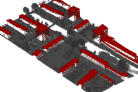
Exporting the data:
In this step, .las files are converted to a 'HDF5 binary data format'. For this step of exporting the data into an intermediate format, use the Prepare Point Cloud Training Data tool in the 3D Analyst extension, available from ArcGIS Pro 2.8 onwards (as shown in figure 1).
The tool needs two LAS datasets, one for the training data and one for the validation data or regions of interest defined by polygons. Next, the block size is set to '50 meters', as our objects of interest will mostly be smaller than that, and the default value of '8192' is used for block point limit.

Figure 1.
Prepare Point Cloud Training Datatool.
Here, all the additional attributes are included in the exported data. Later, a subset of additional attributes like intensity, number of returns, etc. can be selected that will be considered for training.
After the export is completed at the provided output path, the folder structure of the exported data will have two folders, each with converted HDF files in them (as shown in figure 2). The exported training and validation folders will also contain histograms of the distributions of data that provide additional understanding and can help in tweaking the parameters that are being used in the workflow.

Figure 2. Exported data.
Preparing the data:
For prepare_data(), deciding the value of batch_size will depend on either the available RAM or VRAM, depending upon whether CPU or GPU is being used. transforms can also be used for introducing rotation, jitter, etc. to make the dataset more robust. data.classes can be used to verify what classes the model will be learning about.
The classes_of_interest and min_points parameters can be used to filter out less relevant blocks. These parameters are useful when training a model for SfM-derived or mobile/terrestrial point clouds. In specific scenarios when the 'training data' is not small, usage of these features can result in speeding up the 'training time', improving the convergence during training, and addressing the class imbalance up to some extent.
In this sample notebook X, Y, Z, and intensity are considered for training the model. So, 'intensity' is selected as extra_features. The names of the classes are also defined using class_mapping and will be saved inside the model for future reference.
output_path = r'C:\project\exported_data.pctd'colormap = {'6':[255,69,0], '19':[253,247,83]}data = prepare_data(output_path,
dataset_type='PointCloud',
batch_size=2,
transforms=None,
color_mapping=colormap,
extra_features=['intensity'],
class_mapping={'6':'building','19':"background"})data.classesVisualization of prepared data
show_batch() helps in visualizing the exported data. Navigation tools available in the graph can be used to zoom and pan to the area of interest.
data.show_batch(rows=1)
Figure 3. Visualization of batch.
Training the model
First, the PointCNN model object is created, utilizing the prepared data.
pc = PointCNN(data)Next, the lr_find() function is used to find the optimal learning rate that controls the rate at which existing information will be overwritten by newly acquired information throughout the training process. If no value is specified, the optimal learning rate will be extracted from the learning curve during the training process.
pc.lr_find()
0.0003311311214825911
The fit() method is used to train the model, either applying a new 'optimum learning rate' or the previously computed 'optimum learning rate' (any other user-defined learning rate can also be used.).
If early_stopping is set to 'True', then the model training will stop when the model is no longer improving, regardless of the epochs parameter value specified. The best model is selected based on the metric selected in the monitor parameter. A list of monitor's available metrics can be generated using the available_metrics property.
An 'epoch' means the dataset will be passed forward and backward through the neural network one time, and if Iters_per_epoch is used, a subset of data is passed per epoch. To track information like gradients, losses, metrics, etc. while the model training is in progress, tensorboard can be set to 'True'.
pc.available_metrics['valid_loss', 'accuracy', 'precision', 'recall', 'f1']
pc.fit(30, 0.0003311311214825911, monitor='f1', tensorboard=True, early_stopping=True)Monitor training on Tensorboard using the following command: 'tensorboard --host=DEMOPC01 --logdir="C:\project\exported_data.pctd\training_log"'
| epoch | train_loss | valid_loss | accuracy | precision | recall | f1 | time |
|---|---|---|---|---|---|---|---|
| 0 | 0.414868 | 0.327828 | 0.961552 | 0.580412 | 0.500773 | 0.491984 | 51:46 |
| 1 | 0.180299 | 0.152622 | 0.961906 | 0.558456 | 0.508025 | 0.498137 | 52:12 |
| 2 | 0.134608 | 0.114754 | 0.962637 | 0.732194 | 0.521849 | 0.530341 | 53:02 |
| 3 | 0.115696 | 0.103849 | 0.965638 | 0.740362 | 0.578991 | 0.606499 | 55:15 |
| 4 | 0.101456 | 0.083759 | 0.972504 | 0.758468 | 0.641700 | 0.676384 | 53:07 |
| 5 | 0.091657 | 0.078313 | 0.978683 | 0.764146 | 0.716316 | 0.732368 | 53:41 |
| 6 | 0.077390 | 0.055922 | 0.984198 | 0.810564 | 0.738881 | 0.767787 | 1:02:30 |
| 7 | 0.062161 | 0.056305 | 0.984254 | 0.809325 | 0.730631 | 0.760365 | 1:05:56 |
| 8 | 0.053943 | 0.040296 | 0.987276 | 0.816530 | 0.765274 | 0.785336 | 1:06:09 |
| 9 | 0.046304 | 0.041236 | 0.986681 | 0.814050 | 0.764801 | 0.783799 | 1:05:47 |
| 10 | 0.041033 | 0.039411 | 0.986772 | 0.809824 | 0.762317 | 0.780635 | 1:05:57 |
| 11 | 0.038530 | 0.037952 | 0.987333 | 0.813191 | 0.774905 | 0.789596 | 1:06:01 |
| 12 | 0.036169 | 0.035585 | 0.988241 | 0.810229 | 0.783942 | 0.792735 | 1:06:32 |
| 13 | 0.035043 | 0.035248 | 0.988394 | 0.806603 | 0.794934 | 0.796639 | 1:08:40 |
| 14 | 0.031592 | 0.032997 | 0.988970 | 0.810221 | 0.795412 | 0.797727 | 1:23:01 |
| 15 | 0.030037 | 0.033721 | 0.988854 | 0.812487 | 0.791296 | 0.796691 | 1:07:23 |
| 16 | 0.028991 | 0.033177 | 0.988686 | 0.846634 | 0.803212 | 0.818482 | 1:07:49 |
| 17 | 0.028008 | 0.044601 | 0.984940 | 0.843427 | 0.806444 | 0.814293 | 1:08:01 |
| 18 | 0.026430 | 0.038030 | 0.987167 | 0.831564 | 0.801976 | 0.808202 | 1:08:20 |
| 19 | 0.026711 | 0.045163 | 0.983954 | 0.800774 | 0.791680 | 0.785958 | 1:08:18 |
| 20 | 0.026958 | 0.058079 | 0.977928 | 0.800937 | 0.782517 | 0.778332 | 1:08:53 |
| 21 | 0.025250 | 0.073019 | 0.980236 | 0.880202 | 0.761289 | 0.796071 | 1:07:13 |
Epoch 22: early stopping
Visualization of results in notebook
show_results() will visualize the results of the model for the same scene as the ground truth. Navigation tools available in the graph can be used to zoom and pan to the area of interest.
The compute_precision_recall() method can be used to compute per-class performance metrics, which are calculated against the validation dataset.
pc.show_results(rows=1)
Figure 4. Visualization of results.
Saving the trained model
The last step related to training is to save the model using the save() method. Along with the model files, this method also saves performance metrics, a graph of training loss vs validation loss, sample results, etc. (as shown in figure 5).

Figure 5. Saved model.
pc.save('building_and_background')WindowsPath('models/building_and_background')Classification using the trained model
For inferencing, Classify Points Using Trained Model tool in the 3D Analyst extension, available from ArcGIS Pro 2.8 onwards, can be used (as shown in figure 6).
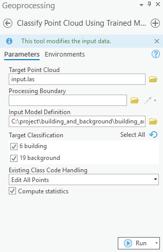
Figure 6.
Classify Points Using Trained Modeltool.
Additional features, like target classification and class preservation in input data, are also available. After the prediction, LAS files will have 'building points', with the class code '6', and the rest of the points will have the class code '19' (referred to as 'Background' in this sample). To visualize the results after the process is completed, the 'Symbology' can be changed to 'class' from the 'Appearance' tab, if not done initially.
Post-processing in ArcGIS Pro and City Engine
There can be multiple unsupervised/semi-supervised workflows to clean the noise and generate building footprints from classified building points. The method used for this work is described below:
We start with PointCNN's classified building points (as shown in figure 7).

Figure 7. Visualization of results in ArcGIS Pro.
Model Builder:
Then using multiple geoprocessing tools in ArcGIS Pro within a model builder, noises are cleaned and building footprints are generated. These footprints are later used to generate multipatches.
The model builder used in this sample can be downloaded from here . The model builder can be used via its tool UI (as shown in figure 8.1), or it can also be used via the model builder wizard in ArcGIS Pro (as shown in figure 8.2). If needed the workflow can be also be edited/customized.

Figure 8.1. Model builder tool UI.

Figure 8.2. Model builder.
The model builder takes filtered 'building points' as 'input' ('LAS filter' can be used for this, as shown in figure 9). In this post-processing pipeline, important prior information is that "no building will have a very small area". This information is used to apply 'area-based thresholding' using Select by Attribute and reduce the noise polygons generated from noise points. If needed, this 'area-based threshhold value' can be changed by editing the model builder.

Figure 9. Filtering of points.
After smoothening and regularizing the polygons (as shown in figure 10), Zonal Statistics is used to populate the footprint polygon's attribute table with 'avg. building height'. Later, other information like building type, no. of floors, etc. are also added, which are later used by City Engine's rule package to generate better digital twins of buildings.

Figure 10. Building footprint.
Lastly, these footprints are used to generate realistic 3D models/multipatches using City Engine's rule packages. Where Features From CityEngine Rules is used. The rule package used in this sample can be downloaded from here. It is created using City Engine's CGA rules, and the 'connection attributes' can be noted down from City Engine (as shown in figure 11).

Figure 11. City Engine's CGA rules.
Visualization of results in ArcGIS Pro
Building Multipatches are the final output of this sample (as shown in figure 12). The output is very close to real-world buildings from the 'area of interest', in terms of 'accurate depiction' and 'aesthetics'.

Figure 12. Building Multipatches.
This web scene has the final and intermediate outputs related to the illustrated test data in this notebook. It can also be accessed via its itemId, as shown below.
results = gis.content.get('908161d7ebfe49e3b318aa7139968ba5')
results
Conclusion
This notebook has walked us through an end-to-end workflow for training a deep learning model for point cloud classification and generating digital twins of real-world objects from the classified points. A similar approach can be applied to classify other objects of interest like trees, traffic lights, wires, etc.
References
- AHN3 data used in this sample is licensed under the Creative Commons Zero license.