- 🔬 Data Science
- 🥠 Deep Learning and Feature Classifier
Introduction and methodology
This sample notebook demonstrates the use of deep learning capabilities in ArcGIS to perform feature categorization. Specifically, we are going to perform automated damage assessment of homes after the devastating Woolsey fires. This is a critical task in damage claim processing, and using deep learning can speed up the process and make it more efficient. The workflow consists of three major steps: (1) extract training data, (2) train a deep learning feature classifier model, (3) make inference using the model.
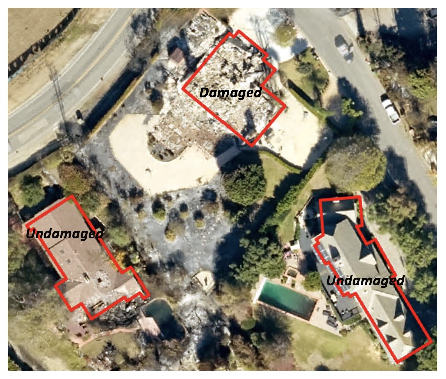
Figure 1. Feature classification example
Methodology

Figure 2. Methodology
Part 1 - Export training data for deep learning
To export training data for feature categorization, we need two input data:
- An input raster that contains the spectral bands,
- A feature class that defines the location (e.g. outline or bounding box) and label of each building.
Import ArcGIS API for Python and get connected to your GIS
import os
from pathlib import Path

import arcgis
from arcgis import GIS
from arcgis import learn, create_buffers
from arcgis.raster import analytics, Raster
from arcgis.features.analysis import join_features
from arcgis.learn import prepare_data, FeatureClassifier, classify_objects,  Model, list_models
arcgis.env.verbose = True
gis = GIS('home')
gis_ent = GIS('https://pythonapi.playground.esri.com/portal', 'arcgis_python', 'amazing_arcgis_123')Prepare data that will be used for training data export
A building footprints feature layer will be used to define the location and label of each building.
building_footprints = gis.content.search('buildings_woolsey', item_type='Feature Layer Collection')[0]
building_footprints
We will buffer the building footprints layer for 150m using create_buffers . With 150m buffer, when the training data will be exported it will cover the surrounding of houses which will help the model to understand the difference between damaged and undamaged houses.
building_buffer = arcgis.create_buffers(building_footprints,
                                        distances=[150],
                                        units='Meters',
                                        dissolve_type='None',
                                        ring_type='Disks',
                                        side_type='Full',
                                        end_type='Round',
                                        output_name='buildings_buffer'+str(datetime.now().microsecond),
                                        gis=gis_ent)
building_buffer
building_buffer.share(everyone=True){'results': [{'itemId': '44f59ce43bdc43afb8bf8d085b2664f5',
'success': True,
'notSharedWith': []}]}An aerial imagery of West Malibu will be used as input raster that contains the spectral bands. This raster will be used for exporting the training data.
input_raster = Raster("https://pythonapi.playground.esri.com/ra/rest/services/Hosted/raster_for_training_damage_classifier/ImageServer",
                        gis=gis_ent,
                        engine="image_server")
input_raster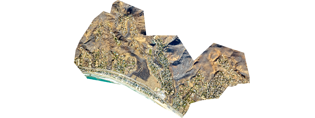
Specify a folder name in raster store that will be used to store our training data
ds = analytics.get_datastores(gis=gis_ent)
ds
<DatastoreManager for https://pythonapi.playground.esri.com/ra/admin>
ds.search(types="rasterStore") [<Datastore title:"/rasterStores/RasterDataStore" type:"rasterStore">]
rasterstore = ds.get('/rasterStores/RasterDataStore')
rasterstore
<Datastore title:"/rasterStores/RasterDataStore" type:"rasterStore">
samplefolder = "feature_classifier_sample"+str(datetime.now().microsecond)
samplefolder
'feature_classifier_sample471203'
output_folder = rasterstore.datapath + "/" + samplefolder
output_folder
'/rasterStores/RasterDataStore/feature_classifier_sample471203'
Export training data using arcgis.learn
Now ready to export training data using the export_training_data() method in arcgis.learn module. In addtion to feature class, raster layer, and output folder, we also need to specify a few other parameters such as tile_size (size of the image chips), stride_size (distance to move each time when creating the next image chip), chip_format (TIFF, PNG, or JPEG), metadata_format (how we are going to store those training labels). Note that unlike Unet and object detection, the metadata is set to be Labeled_Tiles here. More detail can be found here.
Depending on the size of your data, tile and stride size, and computing resources, this operation can take a while. In our experiments, this took 15mins~2hrs. Also, do not re-run it if you already run it once unless you would like to update the setting.
We will export the training data for a small sub-region of our study area and the whole study area will be used for inferencing of results. We will create a map widget, zoom in to the western corner of our study area and get the extent of the zoomed in map. We will use this extent in Export training data using deep learning function.
export = learn.export_training_data(input_raster=input_raster,
                                    output_location=output_folder,
                                    input_class_data=building_buffer.layers[0],
                                    classvalue_field = "class_ecode",
                                    chip_format="TIFF",
                                    tile_size={"x":600,"y":600},
                                    stride_size={"x":0,"y":0},
                                    metadata_format="Labeled_Tiles",
                                    context={"startIndex": 0, "exportAllTiles": False, "cellSize": 0.1},
                                    gis = gis_ent)
Part 2 - Model training
If you've already done part 1, you should already have the training chips. Please change the path to your own export training data folder that contains "images" and "labels" folder.
training_data = gis.content.get('14f3f9421c6b4aa3bf224479c0eaa4f9')
training_data
filepath = training_data.download(file_name=training_data.name)import zipfile
with zipfile.ZipFile(filepath, 'r') as zip_ref:
zip_ref.extractall(Path(filepath).parent)data_path = Path(os.path.join(os.path.splitext(filepath)[0]))data = prepare_data(data_path, {1:'Damaged', 2:'Undamaged'}, chip_size=600, batch_size=16)Visualize training data
To get a sense of what the training data looks like, arcgis.learn.show_batch() method randomly picks a few training chips and visualize them.
data.show_batch()
Load model architecture
Now the building classification problem has become a standard image classfication problem. By default arcgis.learn uses Resnet34 as its backbone model followed by a softmax layer.
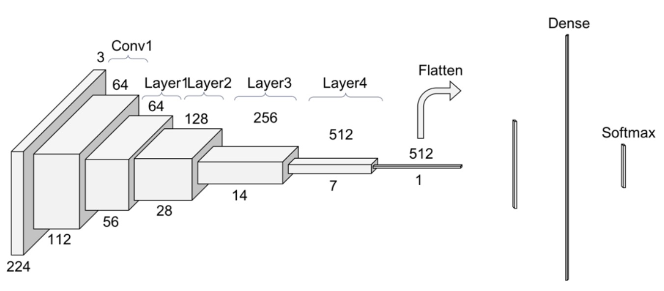
Figure 2. Resnet34 architecture [1]
model = FeatureClassifier(data)Train a model through learning rate tuning and transfer learning
Learning rate is one of the most important hyperparameters in model training. Here we explore a range of learning rates to guide us to choose the best one.
# The users can visualize the learning rate of the model with comparative loss. This case - loss rate decreases, so we are detecting more n more objects as it learns more
lr = model.lr_find()
lr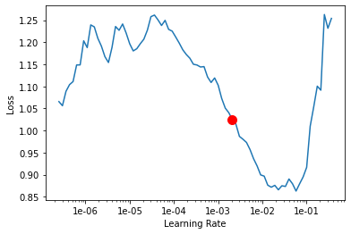
0.0020892961308540407
Based on the learning rate plot above, we can see that the loss going down most dramatically at 1e-2. Therefore, we set learning rate to be to 1e-2. Let's start with 10 epochs for the sake of time.
model.fit(epochs=15, lr=1e-2)| epoch | train_loss | valid_loss | accuracy | time |
|---|---|---|---|---|
| 0 | 0.797712 | 0.167357 | 0.915493 | 00:44 |
| 1 | 0.486395 | 0.355162 | 0.915493 | 00:44 |
| 2 | 0.367514 | 0.103459 | 0.943662 | 00:44 |
| 3 | 0.381270 | 0.743959 | 0.859155 | 00:44 |
| 4 | 0.379432 | 0.819107 | 0.873239 | 00:44 |
| 5 | 0.473011 | 0.116100 | 0.971831 | 00:44 |
| 6 | 0.439557 | 0.431866 | 0.901408 | 00:44 |
| 7 | 0.329892 | 0.470854 | 0.901408 | 00:44 |
| 8 | 0.273802 | 0.209666 | 0.943662 | 00:44 |
| 9 | 0.240444 | 0.065070 | 0.971831 | 00:45 |
| 10 | 0.219831 | 0.219598 | 0.943662 | 00:45 |
| 11 | 0.181914 | 0.042719 | 0.985915 | 00:45 |
| 12 | 0.144126 | 0.068111 | 0.971831 | 00:44 |
| 13 | 0.127985 | 0.066318 | 0.971831 | 00:44 |
| 14 | 0.100624 | 0.061496 | 0.971831 | 00:44 |
Visualize classification results in validation set
Now we have the model, let's look at how the model performs.Now that we have the model, let's evaluate its performance. By setting gradcam = True, we can visualize which parts of the image the model is focusing on during classification. This helps improve explainability by showing which regions contribute most to the model's decisions.
model.show_results(rows=10,gradcam = True)
As we can see, with only 15 epochs, we are already seeing reasonable results. Further improvment can be acheived through more sophisticated hyperparameter tuning. Let's save the model for further training or inference later. The model should be saved into a models folder in your folder. By default, it will be saved into your data_path that you specified in the very beginning of this notebook.
When saving the model, setting gradcam = True not only enables Grad-CAM visualizations getting stored in the model.metrics file on the validation data.
This is especially useful when using the model later in ArcGIS Pro with the Classify Objects Using Deep Learning toolbox. In ArcGIS Pro, this setting adds a parameter called explainability_map to the model arguments. If you set explainability_map=True, Grad-CAM heatmaps will be generated and attached to each classified feature in the attribute table. These can then be easily visualized using pop-ups, helping you understand which regions of the image influenced the model’s predictions
model.save(r'damage_classifier_15e', publish=True, gis=gis_ent,gradcam = True)Published DLPK Item Id: 6a71b3fe09a84d02ba24f48319760564
WindowsPath('D:/data/damage_classifier_15e')Accuracy assessment
arcgis.learn provides the plot_confusion_matrix() function that plots a confusion matrix of the model predictions to evaluate the model's accuracy.
model.plot_confusion_matrix()
The confusion matrix validates that the trained model is learning to classify and differentiate between damaged and undamaged houses. The diagonal numbers show the number of scenes correctly classified as their respective categories
Part 3 - Inference and post processing
Now we have the model ready, let's apply the model to a new feature class with a few new buildings and see how it performs.
fc_model_package = gis_ent.content.search("finetuned_damage_classifier_model owner:api_data_owner", item_type='Deep Learning Package')[0]
fc_model_packageNow we are ready to install the model. Installation of the deep learning model item will unpack the model definition file, model file and the inference function script, and copy them to "trusted" location under the Raster Analytic Image Server site's system directory.
fc_model = Model(fc_model_package)fc_model.install()fc_model.query_info()We will use Classify Objects Using Deep Learning for inferencing the results. The parameters required to run the function are:
in_raster:The input raster dataset to classify. The input can be a single raster or multiple rasters in a mosaic dataset, an image service, or a folder of images.out_feature_class: The output feature class that will contain geometries surrounding the objects from the input feature class, as well as a field to store the classification label.in_model_definition: It contains the path to the deep learning binary model file, the path to the Python raster function to be used, and other parameters such as preferred tile size or padding.in_features: input feature class represents a single object. If no input feature class is specified, the tool assumes that each input image contains a single object to be classified.class_label_field: The name of the field that will contain the classification label in the output feature class. If no field name is specified, a new field called ClassLabel will be generated in the output feature class.
raster_for_inferencing = gis_ent.content.search('bc005b5349b6475aaf331d9f39e89466')[0]
raster_for_inferencinginferenced_lyr = classify_objects(input_raster=raster_for_inferencing,
model = fc_model,
model_arguments={'batch_size': 4}
input_features=building_buffer.layers[0],
output_name="inferenced_layer_fc"+str(datetime.now().microsecond),
class_value_field='status',
context={'cellSize': 0.5, 'processorType':'GPU'},
gis=gis_ent)
inferenced_lyr
We can load the inference layer into a spatially enabled dataframe to examine the inference result. As we can see, all sample buildings are classified correctly with high confidence.
import pandas as pd
from arcgis.features import GeoAccessor, GeoSeriesAccessor

sdf = pd.DataFrame.spatial.from_layer(inferenced_lyr.layers[0])
sdf[['objectid', 'type', 'status', 'confidence_classifyobjects']].head(10)| objectid | type | status | confidence_classifyobjects | |
|---|---|---|---|---|
| 0 | 1 | Courtyard | Undamaged | 0.999948 |
| 1 | 2 | Courtyard | Undamaged | 0.999177 |
| 2 | 3 | Courtyard | Undamaged | 0.999988 |
| 3 | 4 | Courtyard | Undamaged | 0.999957 |
| 4 | 5 | Courtyard | Undamaged | 0.999875 |
| 5 | 6 | Courtyard | Undamaged | 0.999691 |
| 6 | 7 | Courtyard | Damaged | 0.990788 |
| 7 | 8 | Courtyard | Undamaged | 0.954395 |
| 8 | 9 | Courtyard | Undamaged | 0.999292 |
| 9 | 10 | Courtyard | Undamaged | 0.999616 |
The next step is to join the inferenced_lyr with building_footprints so that the building_footprints layer will have the status column. We will use the output layer of join features function for visualization of results in map widget.
final_lyr = arcgis.features.analysis.join_features(building_footprints,
                                                   inferenced_lyr,
                                                   attribute_relationship=['{"targetField":"building_i","operator":"equal","joinField":"building_i"}'],
                                                   join_operation='JoinOneToOne',
                                                   output_name='bfootprint_withstatus'+str(datetime.now().microsecond),
                                                   gis=gis_ent)
final_lyrWe can see the results in the webmap, click on the webmap a new tab will open which will show the classified building footprint layer overlayed on the aerial imagery. You can also add your inferenced layer to this webmap.
webmap = gis.content.search('woolsey_building_damage', outside_org=True)[0]
webmap
Part 4 - Explainbility Map inferencing in ArcGIS Pro
This section demonstrates how to perform explainability map inferencing using ArcGIS Pro tools.
It specifically shows how to generate Grad-CAM outputs by running the Classify Objects Using Deep Learning tool.
Load the saved model in Classify Objects Using Deep Learning. Set the model arguments 'explainbility_map = True' . Click on Run.

After the Classify Objects Using Deep Learning tool finishes processing, select any feature from the output layer in the map view. You can either click directly on a feature to open its pop-up window, or open the Attribute Table for the output layer, right-click on a row, and select Pop-up to view the feature details. The classification results, along with any explainability outputs (such as Grad-CAM maps), will be accessible through these views like below.

As we can observe, the feature above has been classified as "damaged." The Grad-CAM output highlights the regions the model focused on when making this classification, clearly indicating that the model is prioritizing the damaged area in its decision-making process.
Conclusion
In this notebook, we have covered a lot of ground. In part 1, we discussed how to export training data for deep learning using ArcGIS python API. In part 2, we demonstrated how to prepare the input data, train a feature classifier model, visualize the results, as well as apply the model to an unseen image. Then we covered how to installation of model, inferencing and post processing of inferenced results to make it production-ready in part 3. The same workflow can be applied to many other use cases. For example, when we know the locations of swimming pools, we can use it to indentify which ones are dirty and not being properly maintained. In Part 4, we demonstrated how to view Grad-CAM results, which play a crucial role in understanding the model's decision-making process. This approach is not only valuable for model training and refinement (using 'show_results(gradcam=True)'), but also for explaining the model's predictions (through the Classify Objects Using Deep Learning tool).
Reference
[1] Ruiz Pablo, Understanding and Visualizing ResNets, https://towardsdatascience.com/understanding-and-visualizing-resnets-442284831be8, Accessed 2 September 2019.