- 🔬 Data Science
- 🥠 Deep Learning and Object classification
Introduction
In this sample notebook, we will be using the ArcGIS API for Python for training an object classification model on image data from an external source and using that model for inferencing in ArcGIS Pro.
For this example, we will be using the RESISC45 Dataset, which is a publicly available benchmark for Remote Sensing Image Scene Classification (RESISC) created by Northwestern Polytechnical University (NWPU). This dataset contains 31,500 images covering 45 scene classes, with 700 images in each class.
We will be using this dataset to train a FeatureClassifier model that will classify satellite image tiles in the 45 scene classes specified in the dataset.
Necessary imports
import os, json
from arcgis.learn import prepare_data, FeatureClassifier
Download & setting up training data
Since the RESISC45 Dataset is publically available, we will download the data from the Tensorflow website.
The name of the dataset we will be downloading is NWPU-RESISC45.rar
After the data has been downloaded, follow the steps below to prepare the model for the FeatureClassifier.
- Extract the .rar file
- Create a folder named images and move all the 45 folders (correspoding to each class in the dataset) into the images folder

Next, we will create an data_path variable containing the path of the images folder.
data_path = os.path.join(os.getcwd(), "NWPU-RESISC45")Train the model
arcgis.learn provides the ability to determine the class of each feature in the form of a FeatureClassifier model. To learn more about how it works and its potential use cases, see this guide - "How feature classifier works?".
Prepare data
Here, we will specify the path to our training data and a few hyperparameters.
path: path of the folder/list of folders containing training data.dataset_type: The type of dataset getting passed to the Feature Classifier.batch_size: Number of images your model will train on each step inside an epoch. This directly depends on the memory of your graphic card. 128 worked for us on a 32GB GPU.
Since we are using the dataset from external source for training our FeatureClassifier, we will be using Imagenet as dataset_type.
data = prepare_data(
    path=data_path, dataset_type="Imagenet", batch_size=128, val_split_pct=0.2
)
Visualize training data
To get a sense of what the training data looks like, the show_batch() method randomly picks a few training chips and visualizes them.
rows: Number of rows to visualize
data.show_batch(rows=5)
Load model architecture
model = FeatureClassifier(data, oversample=True)Find an optimal learning rate
Learning rate is one of the most important hyperparameters in model training. The ArcGIS API for Python provides a learning rate finder that automatically chooses the optimal learning rate for you.
lr = model.lr_find()
Fit the model
We will train the model for a few epochs with the learning rate we have found. For the sake of time, we can start with 20 epochs.
model.fit(20, lr=lr)| epoch | train_loss | valid_loss | accuracy | time |
|---|---|---|---|---|
| 0 | 3.849639 | 2.303129 | 0.393016 | 05:32 |
| 1 | 1.891675 | 0.922773 | 0.741905 | 04:23 |
| 2 | 1.015606 | 0.534618 | 0.840635 | 04:05 |
| 3 | 0.686829 | 0.421678 | 0.870952 | 03:57 |
| 4 | 0.508045 | 0.351383 | 0.891746 | 03:53 |
| 5 | 0.418271 | 0.315520 | 0.900635 | 03:51 |
| 6 | 0.376608 | 0.286548 | 0.912063 | 03:52 |
| 7 | 0.319486 | 0.281573 | 0.911270 | 03:53 |
| 8 | 0.295100 | 0.260070 | 0.919048 | 03:51 |
| 9 | 0.278306 | 0.244136 | 0.922381 | 03:51 |
| 10 | 0.263577 | 0.235160 | 0.922381 | 03:51 |
| 11 | 0.227998 | 0.231522 | 0.925238 | 03:52 |
| 12 | 0.205606 | 0.223483 | 0.929048 | 03:51 |
| 13 | 0.209035 | 0.222402 | 0.929524 | 03:51 |
| 14 | 0.195011 | 0.215549 | 0.930159 | 03:51 |
| 15 | 0.188278 | 0.213108 | 0.930317 | 03:52 |
| 16 | 0.178093 | 0.209075 | 0.930794 | 03:51 |
| 17 | 0.176601 | 0.208589 | 0.932540 | 03:51 |
| 18 | 0.188212 | 0.205964 | 0.933492 | 03:51 |
| 19 | 0.175853 | 0.204608 | 0.933016 | 03:51 |
Here only after 20 epochs both training and validation losses have decreased considerably, indicating that the model is learning to classify image scenes.
Visualize results in the validation set
It is a good practice to see the results of the model viz-a-viz ground truth. The code below picks random samples and shows us ground truth and model predictions side by side. This enables us to preview the results of the model within the notebook.
model.show_results(rows=4)
Here, with only 20 epochs, we can see reasonable results.
Accuracy assessment
arcgis.learn provides the plot_confusion_matrix() function that plots a confusion matrix of the model predictions to evaluate the model's accuracy.
model.plot_confusion_matrix()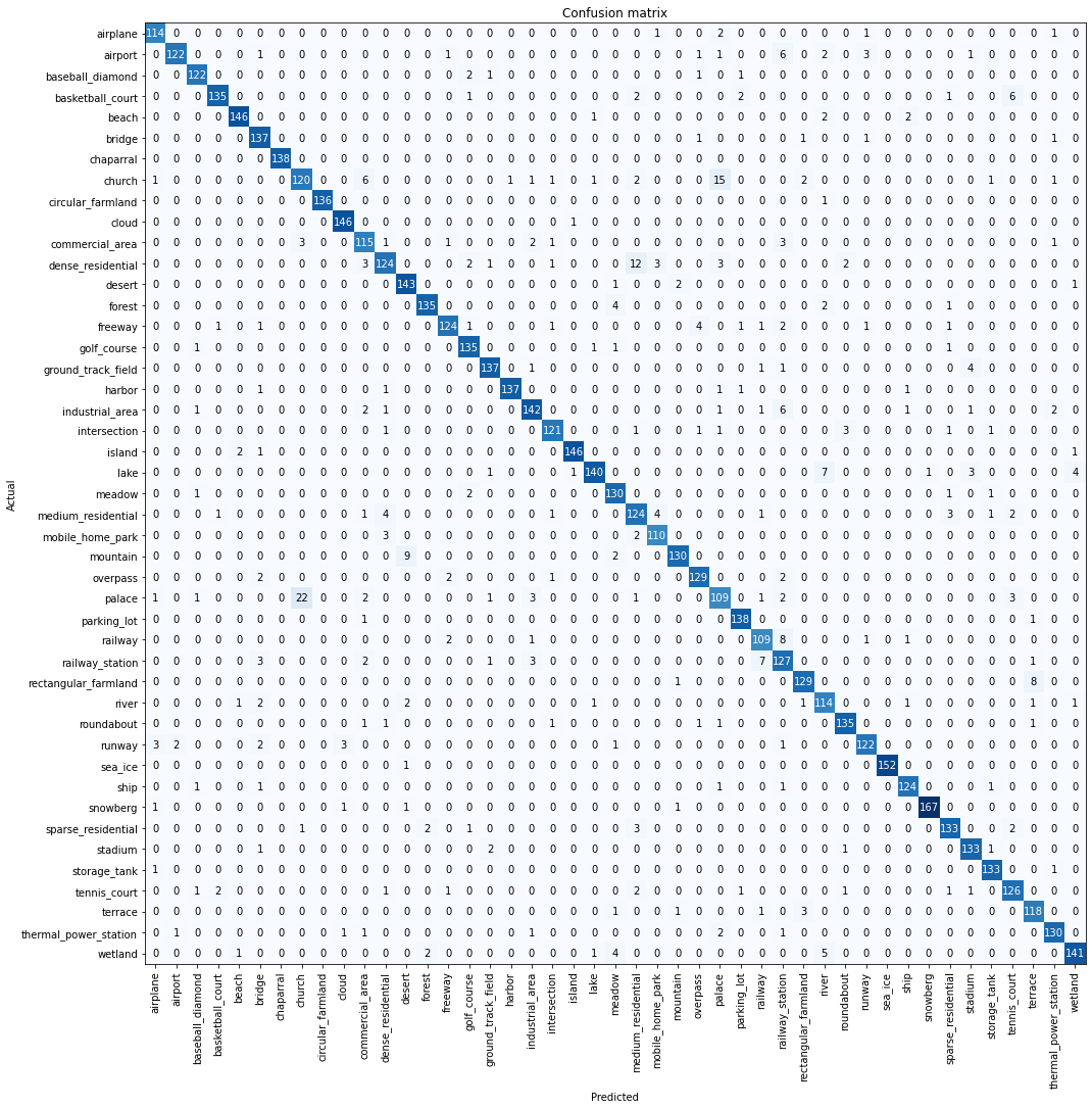
The confusion matrix validates that the trained model is learning to classify scenes to different classes. The diagonal numbers show the number of scenes correctly classified as their respective categories.
Save the model
Now, we will save the model that we trained as a 'Deep Learning Package' ('.dlpk' format). A Deep Learning package is the standard format used to deploy deep learning models on the ArcGIS platform.
We will use the save() method to save the trained model. By default, it will be saved to the 'models' sub-folder within our training data folder.
model_name = "Nwpu_model1"
model.save(model_name)WindowsPath('D:/NWPU/NWPU-RESISC45/models/Nwpu_model1')Model inference
Before using the model for inference, we need to make some changes in the model_name.emd file. You can learn more about this file here.
By default, in the EMD file, the CropSizeFixed is set to 1. We need to change the CropSizeFixed to 0 so that the size of tiles cropped around the feature are not fixed.
with open(
    os.path.join(data_path, "models", model_name, model_name + ".emd"), "r+"
) as emd_file:
    data = json.load(emd_file)
    data["CropSizeFixed"] = 0
    emd_file.seek(0)
    json.dump(data, emd_file, indent=4)
    emd_file.truncate()
For us to perform inferencing in ArcGIS Pro, we need to create a feature class on the map using either the Create Feature Class tool or the Create Fishnet tool, for an area that has not already seen by the model.
We have also provided the Feature Class and the Model trained on the NWPU Dataset for reference. You can directly download these to run your own experiments from the links below.
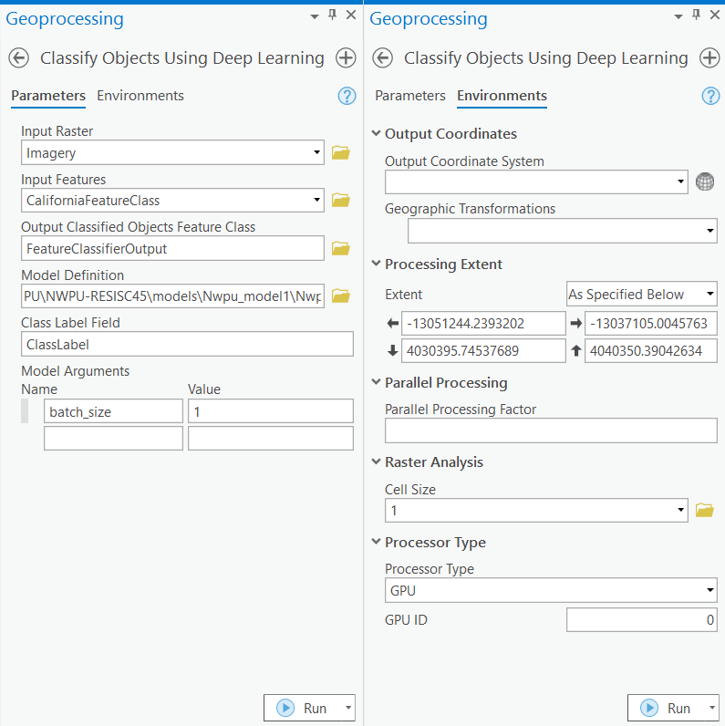
Now, we will use the Classify Objects Using Deep Learning tool for inferencing the results. The parameters required to run the function are:
Input Raster: High_Resolution_ImageryInput Features: Output from theCreate Feature ClassorCreate Fishnettool.Output CLassified Objects Feature Class: Output feature class.Model Definition: Emd file of the model that we trained.Class Label Field: Field name that will contain the detected class number.Environments: Set optimumCell Size,Processing ExtentandProcessor Type.
We have investigated and found that a Cell Size of 1m/pixel works best for this model.
Results
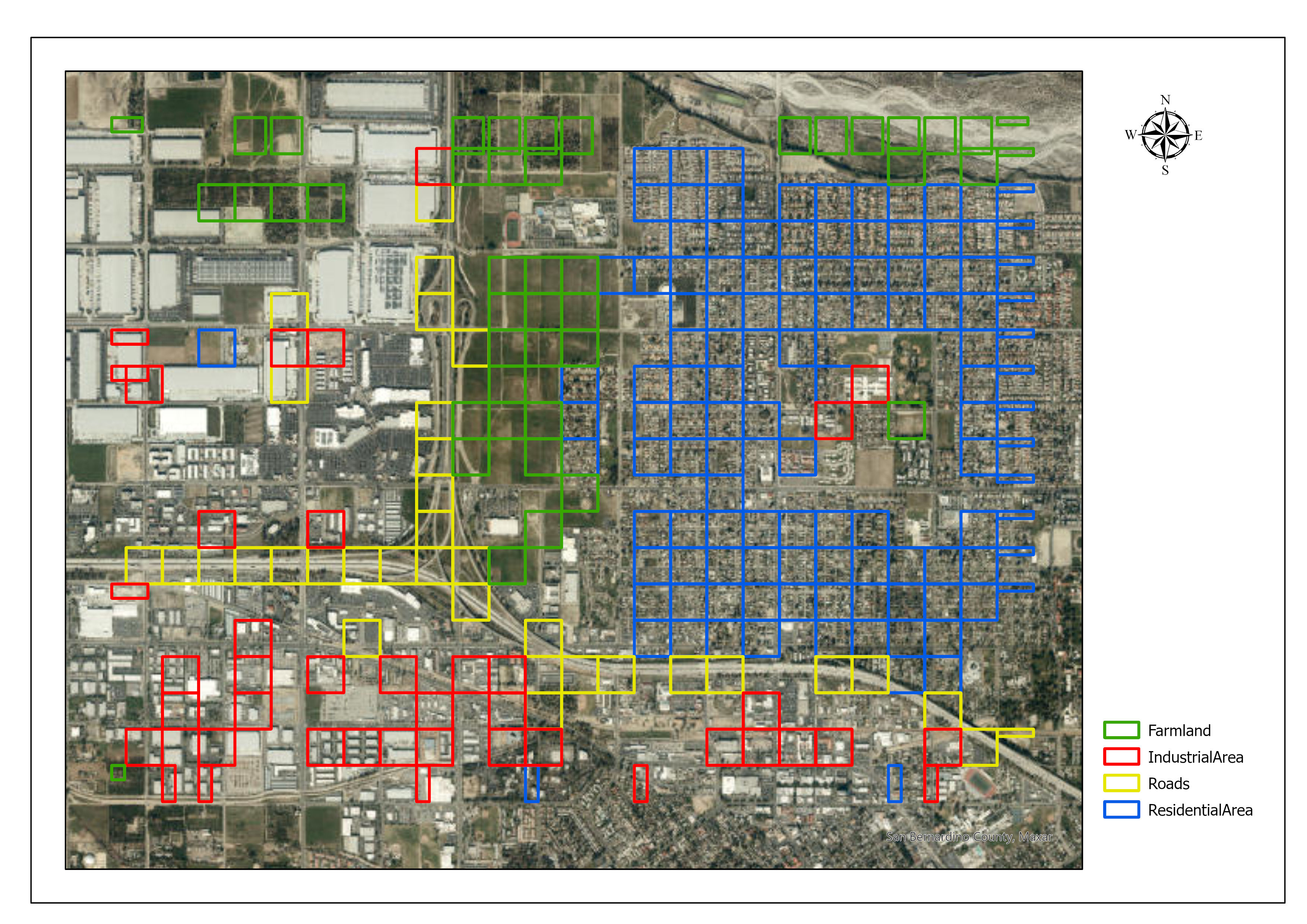
We selected an area that had not been seen by the model and generated the features in it using the Create Feature Class tool. We then used our model for classification. Below are the results.
We also created a fishnet using the Create Fishnet tool that we then fed to our model for classification. We can use this technique to create preliminary data about the image. Based on the output, we can make inferences about the image, such as the total of residential areas, industrial areas in an image, etc. Below is the map that we created from the results.
Conclusion
In this notebook, we demonstrated how to use the FeatureClassifier model from the ArcGIS API for Python to classify image scenes using training data from an external source.
References
- Citation : `@article{cheng2017remote, title={Remote sensing image scene classification: Benchmark and state of the art}, author={Cheng, Gong and Han, Junwei and Lu, Xiaoqiang}, journal={Proceedings of the IEEE}, volume={105}, number={10}, pages={1865--1883}, year={2017}, publisher={IEEE}
}`