Introduction
In part-1 of this guide series, we started with an introduction to the Spatially enabled DataFrame (SeDF), the spatial and geom namespaces, and looked at a quick example of SeDF in action. In this part of the guide series, we will look at how GIS data can be accessed from various data formats using SeDF.
GIS users work with different vector-based spatial data formats, like published layers on remote servers (web layers) and local data. The Spatially enabled DataFrame allows the users to read, write, and manipulate spatial data by bringing the data in-memory.
The SeDF integrates with Esri's ArcPy site-package, as well as the open source pyshp, shapely and fiona packages. This means that the SeDF can use either shapely or arcpy geometry engines to provide you with options for easily working with geospatial data, regardless of your platform. The SeDF transforms the data into the formats you desire, allowing you to use Python functionality to analyze and visualize geographic information.
Data can be read and scripted to automate workflows and be visualized on maps in a Jupyter notebooks. Let's explore the options available for accessing GIS data with the versatile Spatially enabled DataFrame.
The data used in this guide is available as an item. We will start by importing some libraries and downloading and extracting the data needed for the analysis in this guide.
# Import Libraries
import pandas as pd
from arcgis.features import GeoAccessor, GeoSeriesAccessor
from arcgis.gis import GIS
from IPython.display import display
import zipfile
import os
import shutil
# Create a GIS connection
gis = GIS()
agol_gis = GIS("https://www.arcgis.com", "arcgis_python", "amazing_arcgis_123")# Get the data item
data_item = gis.content.get('c7140ae3d7ae4fd0817181461019aa75')
data_item
The cell below downloads and extracts the data from the data item to your machine.
# Download and extract the data
def unzip_data():
    """
    This function:
    - creates a directory `sedf_data` to download the data from the item
    - downloads the item as `sedf_guide_data.zip` file in the sedf_data directory
    - unzips and extracts the data to '.\sedf_data\cities'.
    """
    try:

        # path to downloaded data folder
        data_dir = os.path.join(os.getcwd(), 'sedf_data')

        # remove existing cities directory if exists
        if os.path.isdir(data_dir):
            shutil.rmtree(data_dir)
            print(f'Removed existing data directory')
        else:
            os.makedirs(data_dir)

        data_item.download(data_dir)    # download the data item
        # path to zipped file inside data folder
        zipped_file_path = os.path.join(data_dir, 'sedf_guide_data.zip')

        # unzip the data
        zip_ref = zipfile.ZipFile(zipped_file_path, 'r')
        zip_ref.extractall(data_dir)
        zip_ref.close()

        # path to new cities directory
        cities_dir = os.path.join(data_dir, 'cities')
        print(f'Dataset unzipped at: {os.path.relpath(cities_dir)}')

    except Exception as e:
        print(f'Error unzipping file: {e}')


# Extract data
unzip_data()
Removed existing data directory Dataset unzipped at: sedf_data\cities
Accessing GIS Data
The Spatially enabled DataFrame reads from many sources, including Feature layers, Feature classes, Shapefiles, Pandas DataFrames and more. Let's dive into the details of accessing GIS data from various sources.
Read in Web Feature Layers
Feature layers hosted on ArcGIS Online or ArcGIS Enterprise can be easily read into a Spatially enabled DataFrame using the from_layer() method.
The example below shows how the get() method can be used to retrieve an ArcGIS Online item and how the layers property of an item can be used to access the data.
gis = GIS()
item = gis.content.search(
    "USA Major Cities", item_type="Feature layer", outside_org=True)[0]
item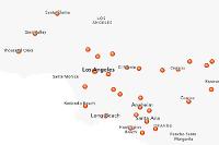
# Obtain the first feature layer from the item
flayer = item.layers[0]

# Use the `from_layer` static method in the 'spatial' namespace on the Pandas' DataFrame
sdf = pd.DataFrame.spatial.from_layer(flayer)

# Check shape
sdf.shape
(3886, 50)
# Check first few records
sdf.head()| AGE_10_14 | AGE_15_19 | AGE_20_24 | AGE_25_34 | AGE_35_44 | AGE_45_54 | AGE_55_64 | AGE_5_9 | AGE_65_74 | AGE_75_84 | ... | PLACEFIPS | POP2010 | POPULATION | POP_CLASS | RENTER_OCC | SHAPE | ST | STFIPS | VACANT | WHITE | |
|---|---|---|---|---|---|---|---|---|---|---|---|---|---|---|---|---|---|---|---|---|---|
| 0 | 1313 | 1058 | 734 | 2031 | 1767 | 1446 | 1136 | 1503 | 665 | 486 | ... | 1601990 | 13816 | 15181 | 6 | 1271 | {"x": -12462673.723706165, "y": 5384674.994080... | ID | 16 | 271 | 13002 |
| 1 | 890 | 817 | 818 | 1799 | 1235 | 1330 | 1143 | 1099 | 721 | 579 | ... | 1607840 | 11899 | 11946 | 6 | 1441 | {"x": -12506251.313993266, "y": 5341537.793529... | ID | 16 | 318 | 9893 |
| 2 | 12750 | 13959 | 16966 | 32135 | 27048 | 29595 | 24177 | 12933 | 12176 | 7087 | ... | 1608830 | 205671 | 225405 | 8 | 33359 | {"x": -12938676.6836459, "y": 5403597.04949123... | ID | 16 | 6996 | 182991 |
| 3 | 790 | 768 | 699 | 1445 | 1136 | 1134 | 935 | 959 | 679 | 464 | ... | 1611260 | 10345 | 10727 | 6 | 1461 | {"x": -12667411.402393516, "y": 5241722.820606... | ID | 16 | 241 | 7984 |
| 4 | 3803 | 3779 | 3687 | 7571 | 5559 | 4744 | 3624 | 4397 | 2296 | 1222 | ... | 1612250 | 46237 | 53942 | 7 | 5196 | {"x": -12989383.674504515, "y": 5413226.487333... | ID | 16 | 1428 | 35856 |
5 rows × 50 columns
# Check type of sdf
type(sdf)
pandas.core.frame.DataFrame
# Access spatial namespace
sdf.spatial.geometry_type
['point']
We can see that the dataset has 3886 records and 50 columns. Inspecting the
typeofsdfobject and accessing thespatialnamespace shows us that a Spatially enabled DataFrame has been created from all the data in the layer.
Memory usage and the query() operation
The from_layer() method will attempt to read all the data from the layer into the memory. This approach works when you are dealing with small datasets. However, when it comes to large datasets, it becomes imperative to use the memory efficiently and query for only what is necessary.
Let's take a look at the memory usage of the existing SeDF using the memory_usage() method from Pandas.
# Check memory usage of current sdf
mem_used = sdf.memory_usage().sum() / (1024**2)  # converting to megabytes
print(f'Shape of data: {sdf.shape}')
print(f'Memory used: {round(mem_used, 2)} MB')
Shape of data: (3886, 50) Memory used: 1.48 MB
We can see that a
SeDFcreated using thefrom_layer()method reads all the data into the memory. So, thesdfobject has 3886 records and 50 columns, and uses 1.48MB memory.
But what if we only needed a small amount of data for our analysis and did not need to bring everything from the layer into the memory? Good question... let's see how we can achieve that.
The query() method is a powerful operation that allows you to use SQL like queries to return only a subset of records. Since the processing is performed on the server, this operation is not restricted by the capacity of your computer.
The method returns a FeatureSet object; however, the return type can be changed to a Spatially enabled DataFrame object by specifying the parameter as_df=True.
Let's subset the data using query(), create a new SeDF, and check the memory usage. We'll use the AGE_45_54 column to query the layer and get a subset of records.
# Filter feature layer records with a query.
sub_sdf = flayer.query(where="AGE_45_54 < 1500", as_df=True)
sub_sdf.shape
(316, 50)
# Check memory usage of current sdf
mem_used = sub_sdf.memory_usage().sum() / (1024**2)  # converting to megabytes
print(f'Memory used is: {round(mem_used, 2)} MB')
Memory used is: 0.12 MB
Now that we are only querying for records where
AGE_45_54 < 1500, the result is a smaller DataFrame with 316 records and 50 columns. Since the processing is performed on the server side, only a subset of data is being saved in the memory reducing usage from 1.48 MB to 0.12 MB.
The query() method allows you to specify a number of optional parameters that may further refine and transform the results. One such key parameter is out_fields. With out_fields, you can subset your data by specifying a list of field names to return.
# Filter feature layer with where and out_fields
out_fields = ['NAME', 'ST', 'POP_CLASS', 'AGE_45_54']
sub_sdf2 = flayer.query(where="AGE_45_54 < 1500",
                        out_fields=out_fields,
                        as_df=True)
sub_sdf2.shape
(316, 6)
# Check head
sub_sdf2.head()| FID | NAME | ST | POP_CLASS | AGE_45_54 | SHAPE | |
|---|---|---|---|---|---|---|
| 0 | 1 | Ammon | ID | 6 | 1446 | {"x": -12462673.723706165, "y": 5384674.994080... |
| 1 | 2 | Blackfoot | ID | 6 | 1330 | {"x": -12506251.313993266, "y": 5341537.793529... |
| 2 | 4 | Burley | ID | 6 | 1134 | {"x": -12667411.402393516, "y": 5241722.820606... |
| 3 | 6 | Chubbuck | ID | 6 | 1494 | {"x": -12520053.904151963, "y": 5300220.333409... |
| 4 | 12 | Jerome | ID | 6 | 1155 | {"x": -12747828.64784961, "y": 5269214.8197742... |
# Check memory usage of current sdf
mem_used = sub_sdf2.memory_usage().sum() / (1024**2)  # converting to megabytes
print(f'Memory used is: {round(mem_used, 2)} MB')
Memory used is: 0.01 MB
Using
out_fields, we have further reduced memory usage by subsetting the data and bringing only necessary information into the memory.
Create SeDF from FeatureSet
As mentioned earlier, the query() method returns a FeatureSet object. The FeatureSet object contains useful information about the data that can be accessed through its various properties.
Let's use the AGE_45_54 column to query the layer to get the result as a FeatureSet and check some its properties.
# Filter feature layer to return a feature set.
fset = flayer.query(where="AGE_45_54 < 1500")
# Check type
type(fset)arcgis.features.feature.FeatureSet
# Check length
len(fset.features)
316
# Check geometry of a feature in the featureset
fset.features[0].geometry
{'x': -12462673.723706165,
'y': 5384674.994080178,
'spatialReference': {'wkid': 102100, 'latestWkid': 3857}}The fields property of a FeatureSet returns a list containing information about each column recorded as a dictionary. Let's use the fields property to access information about the first column.
# Check details of a column in the feature set
fset.fields[0]
{'name': 'FID',
'type': 'esriFieldTypeOID',
'alias': 'FID',
'sqlType': 'sqlTypeInteger',
'domain': None,
'defaultValue': None}Let's get the names of the columns in the data.
# Get column names
f_names = [f['name'] for f in fset.fields]
f_names[:5]
['FID', 'NAME', 'CLASS', 'ST', 'STFIPS']
Now, let's create a Spatially enabled DataFrame from a FeatureSet using the .sdf property.
# Create SeDF from FeatureSet
fset_df = fset.sdf
fset_df.shape
(316, 50)
# Check head
fset_df.head(2)| FID | NAME | CLASS | ST | STFIPS | PLACEFIPS | CAPITAL | POP_CLASS | POPULATION | POP2010 | ... | MARHH_NO_C | MHH_CHILD | FHH_CHILD | FAMILIES | AVE_FAM_SZ | HSE_UNITS | VACANT | OWNER_OCC | RENTER_OCC | SHAPE | |
|---|---|---|---|---|---|---|---|---|---|---|---|---|---|---|---|---|---|---|---|---|---|
| 0 | 1 | Ammon | city | ID | 16 | 1601990 | 6 | 15181 | 13816 | ... | 1131 | 106 | 335 | 3352 | 3.61 | 4747 | 271 | 3205 | 1271 | {"x": -12462673.723706165, "y": 5384674.994080... | |
| 1 | 2 | Blackfoot | city | ID | 16 | 1607840 | 6 | 11946 | 11899 | ... | 1081 | 174 | 381 | 2958 | 3.31 | 4547 | 318 | 2788 | 1441 | {"x": -12506251.313993266, "y": 5341537.793529... |
2 rows × 50 columns
# Check geometry type
fset_df.spatial.geometry_type
['point']
The
spatialnamespace shows that a Spatially enabled DataFrame has been created from aFeatureSet.
Create SeDF from FeatureCollection
Tools within the ArcGIS API for Python often return a FeatureCollection object as a result of some analysis. A FeatureCollection is an in-memory collection of Feature objects with rendering information. Similar to feature layers, feature collections can also be used to store features. With a feature collection, a service is not created to serve out the feature data.
Let's create a SeDF from a FeatureCollection. Here, we:
- Import the Major Ports feature layer.
- Create 5 mile buffers using
create_buffers()tool resulting in a FeatureCollection. - Using the query() method on a FeatureCollection returns a FeatureSet object. We will create a
SeDFfrom the buffered FeatureCollection using the the.sdfproperty of a FeatureSet object returned fromquery().
# Get the ports item
ports_item = gis.content.get("405963eaea24428c9db236ec289760eb")
ports_item
# Get the ports layer
ports_lyr = ports_item.layers[0]
ports_lyr
<FeatureLayer url:"https://geo.dot.gov/server/rest/services/NTAD/Ports_Major/MapServer/0">
# Create buffers
from arcgis.features.use_proximity import create_buffers
ports_buffer50 = create_buffers(
    ports_lyr, distances=[5], units='Miles', gis=agol_gis)
# Check type of result from the analysis
type(ports_buffer50)arcgis.features.feature.FeatureCollection
The
create_buffers()tool resulted in aFeatureCollection.
Now, we will create a SeDF from the FeatureCollection object.
# Create SeDF
sedf_fc = ports_buffer50.query().sdf
sedf_fc.head(2)| OBJECTID_1 | OBJECTID | ID | PORT | PORT_NAME | GRAND_TOTA | FOREIGN_TO | IMPORTS | EXPORTS | DOMESTIC | BUFF_DIST | ORIG_FID | AnalysisArea | SHAPE | |
|---|---|---|---|---|---|---|---|---|---|---|---|---|---|---|
| 0 | 1 | 1 | 124 | C4947 | Unalaska Island, AK | 1652281 | 1236829 | 426251 | 810578 | 415452 | 5 | 1 | 78.528402 | {"rings": [[[-18806114.3995, 7138385.537799999... |
| 1 | 2 | 2 | 85 | C4410 | Kahului, Maui, HI | 3615449 | 20391 | 20391 | 0 | 3595058 | 5 | 2 | 78.528402 | {"rings": [[[-17418472.419, 2388455.4312999994... |
# Check geometry type
sedf_fc.spatial.geometry_type
['polygon']
The
spatialnamespace shows that a Spatially enabled DataFrame has been created from aFeatureCollection.
Read in local GIS data
Local geospatial data, such as Feature classes and shapefiles can be easily accessed using the Spatially enabled DataFrame. The from_featureclass() method can be used to access local data. Let's look at some examples.
Reading a Shapefile
A locally stored shapefile can be accessed by passing the location of the file in the from_featureclass() method.
arcpy, the PyShp package must be present in your current conda environment in order to read shapefiles. To check if PyShp is present, you can run the following in a cell:
!conda list pyshp
To install PyShp, you can run the following in a cell:
!conda install pyshp
# Reading from shape file
shp_df = pd.DataFrame.spatial.from_featureclass(
    location="./sedf_data/cities/cities.shp")
shp_df.shape
(3886, 51)
shp_df.spatial.geometry_type['point']
The
spatialnamespace shows that a Spatially enabled DataFrame has been created from theshapefilestored locally.
Shapefile from a URL
The url of a zipped shapefile can be used to create a SeDF by passing the url as location in the from_featureclass() method. The image below shows how the operation can be performed.
PyShp to be available in the environment.

Reading a Featureclass
A featureclass can be accessed from a File Geodatabase or Mobile Geodatabase (.geodatabase) by passing its location in the from_featureclass() method.
arcpy, the Fiona package must be present in your current conda environment in order to read a featureclass.
To check if Fiona is present, you can run the following in a cell:
!conda list fiona
To install Fiona, you can run the following in a cell:
!conda install fiona
# Reading from FGDB
fcls_df = pd.DataFrame.spatial.from_featureclass(
    location="./sedf_data/cities/cities.gdb/cities")
fcls_df.shape
(3886, 51)
# Check head
fcls_df.head(2)| OBJECTID | age_10_14 | age_15_19 | age_20_24 | age_25_34 | age_35_44 | age_45_54 | age_55_64 | age_5_9 | age_65_74 | ... | placefips | pop2010 | population | pop_class | renter_occ | st | stfips | vacant | white | SHAPE | |
|---|---|---|---|---|---|---|---|---|---|---|---|---|---|---|---|---|---|---|---|---|---|
| 0 | 1 | 1313 | 1058 | 734 | 2031 | 1767 | 1446 | 1136 | 1503 | 665 | ... | 1601990 | 13816 | 15181 | 6 | 1271 | ID | 16 | 271 | 13002 | {"x": -12462673.7237, "y": 5384674.994099997, ... |
| 1 | 2 | 890 | 817 | 818 | 1799 | 1235 | 1330 | 1143 | 1099 | 721 | ... | 1607840 | 11899 | 11946 | 6 | 1441 | ID | 16 | 318 | 9893 | {"x": -12506251.314, "y": 5341537.793499999, "... |
2 rows × 51 columns
# Check geometry type
fcls_df.spatial.geometry_type
['point']
The
spatialnamespace shows that a Spatially enabled DataFrame has been created from thefeatureclassstored locally.
Specify optional parameters
The from_featureclass() method allows users to specify optional parameters when the ArcPy library is available in the current environment. These parameters are:
sql_clause: a pair of SQL prefix and postfix clauses,sql_clause=(prefix,postfix), organized in a list or a tuple can be passed to query specific data. The parameter allows only a small set of operations to be performed. Learn more about the allowed operations here.where_clause: where statement to subset the data. Learn more about it here.fields: to subset the data for specific fields.spatial_filter: a geometry object to filter the results.
arcpy.
Subset data for specific fields
# Subset for fields
fcls_flds = pd.DataFrame.spatial.from_featureclass(location="./sedf_data/cities/cities.gdb/cities",
                                                   fields=['st', 'pop_class'])
fcls_flds.shape
(3886, 3)
# Check head
fcls_flds.head(2)| st | pop_class | SHAPE | |
|---|---|---|---|
| 0 | ID | 6 | {"x": -12462673.7237, "y": 5384674.994099997, ... |
| 1 | ID | 6 | {"x": -12506251.314, "y": 5341537.793499999, "... |
Subset using where_clause
Learn more about how to use where_clause here.
# Subset using where_clause
fcls_whr = pd.DataFrame.spatial.from_featureclass(location="./sedf_data/cities/cities.gdb/cities",
                                                  where_clause="st='ID' and pop_class=6")
fcls_whr.shape
(15, 51)
# Check head
fcls_whr.head(2)| OBJECTID | age_10_14 | age_15_19 | age_20_24 | age_25_34 | age_35_44 | age_45_54 | age_55_64 | age_5_9 | age_65_74 | ... | placefips | pop2010 | population | pop_class | renter_occ | st | stfips | vacant | white | SHAPE | |
|---|---|---|---|---|---|---|---|---|---|---|---|---|---|---|---|---|---|---|---|---|---|
| 0 | 1 | 1313 | 1058 | 734 | 2031 | 1767 | 1446 | 1136 | 1503 | 665 | ... | 1601990 | 13816 | 15181 | 6 | 1271 | ID | 16 | 271 | 13002 | {"x": -12462673.7237, "y": 5384674.994099997, ... |
| 1 | 2 | 890 | 817 | 818 | 1799 | 1235 | 1330 | 1143 | 1099 | 721 | ... | 1607840 | 11899 | 11946 | 6 | 1441 | ID | 16 | 318 | 9893 | {"x": -12506251.314, "y": 5341537.793499999, "... |
2 rows × 51 columns
Subset using fields and where_clause
# Subset using where_clause
flds_whr = pd.DataFrame.spatial.from_featureclass(location="./sedf_data/cities/cities.gdb/cities",
                                                  fields=[
                                                      'st', 'pop_class', 'age_10_14', 'age_15_19'],
                                                  where_clause="st='ID' and pop_class=6")
flds_whr.shape
(15, 5)
# Check head
flds_whr.head(2)| st | pop_class | age_10_14 | age_15_19 | SHAPE | |
|---|---|---|---|---|---|
| 0 | ID | 6 | 1313 | 1058 | {"x": -12462673.7237, "y": 5384674.994099997, ... |
| 1 | ID | 6 | 890 | 817 | {"x": -12506251.314, "y": 5341537.793499999, "... |
Subset using sql_clause
sql_clause can be combined with fields and where_clause to further subset the data. You can learn more about the allowed operations here. Now let's look at some examples.
Prefix sql_clause - DISTINCT operation
# Prefix Sql clause - DISTINCT operation
fcls_sql1 = pd.DataFrame.spatial.from_featureclass(location="./sedf_data/cities/cities.gdb/cities",
                                                   sql_clause=("DISTINCT pop_class", None))

# Check shape
fcls_sql1.shape
(3886, 51)
# Check head
fcls_sql1.head(2)| OBJECTID | age_10_14 | age_15_19 | age_20_24 | age_25_34 | age_35_44 | age_45_54 | age_55_64 | age_5_9 | age_65_74 | ... | placefips | pop2010 | population | pop_class | renter_occ | st | stfips | vacant | white | SHAPE | |
|---|---|---|---|---|---|---|---|---|---|---|---|---|---|---|---|---|---|---|---|---|---|
| 0 | 941 | 1247 | 1213 | 1043 | 2022 | 1692 | 2116 | 1827 | 1187 | 1037 | ... | 0507330 | 15620 | 14771 | 6 | 3006 | AR | 05 | 1303 | 6216 | {"x": -10006810.091, "y": 4290154.581699997, "... |
| 1 | 1405 | 796 | 748 | 754 | 1999 | 1717 | 2062 | 1450 | 760 | 851 | ... | 2466850 | 12677 | 13188 | 6 | 814 | MD | 24 | 281 | 11613 | {"x": -8517714.7855, "y": 4744316.880199999, "... |
2 rows × 51 columns
Postfix sql_clause with specific fields
Here, we will subset the data for the state and population class fields and apply a postfix clause.
# Postfix Sql clause with specific fields
fcls_sql2 = pd.DataFrame.spatial.from_featureclass(location="./sedf_data/cities/cities.gdb/cities",
                                                   fields=['st', 'pop_class'],
                                                   sql_clause=(None, "ORDER BY st, pop_class"))
# Check shape
fcls_sql2.shape
(3886, 3)
# Check head
fcls_sql2.head()| st | pop_class | SHAPE | |
|---|---|---|---|
| 0 | AK | 6 | {"x": -16417572.1606, "y": 9562359.403800003, ... |
| 1 | AK | 6 | {"x": -16455422.2224, "y": 9574022.0224, "spat... |
| 2 | AK | 6 | {"x": -16444303.0276, "y": 9568008.9705, "spat... |
| 3 | AK | 6 | {"x": -14962313.3618, "y": 8031014.926600002, ... |
| 4 | AK | 6 | {"x": -16657118.680399999, "y": 8746757.662600... |
Prefix and Postfix sql_clause with specific fields and where_clause
Here, we will subset the data using where_clause, keep specific fields, and then apply both prefix and postfix clause.
# Prefix and Postfix sql_clause
fcls_sql3_df = pd.DataFrame.spatial.from_featureclass(location="./sedf_data/cities/cities.gdb/cities",
                                                      fields=[
                                                          'st', 'name', 'pop_class', 'age_10_14'],
                                                      where_clause="st='ID'",
                                                      sql_clause=("DISTINCT pop_class", "ORDER BY name"))

# Check Shape
fcls_sql3_df.shape
(22, 5)
# Check head
fcls_sql3_df.head()| st | name | pop_class | age_10_14 | SHAPE | |
|---|---|---|---|---|---|
| 0 | ID | Ammon | 6 | 1313 | {"x": -12462673.7237, "y": 5384674.994099997, ... |
| 1 | ID | Blackfoot | 6 | 890 | {"x": -12506251.314, "y": 5341537.793499999, "... |
| 2 | ID | Boise City | 8 | 12750 | {"x": -12938676.683600001, "y": 5403597.049500... |
| 3 | ID | Burley | 6 | 790 | {"x": -12667411.4024, "y": 5241722.820600003, ... |
| 4 | ID | Caldwell | 7 | 3803 | {"x": -12989383.6745, "y": 5413226.487300001, ... |
Using spatial_filter
spatial_filter can be used to query the results by using a spatial relationship with another geometry. The spatial filtering is even more powerful when integrated with Geoenrichment. Let's use this approach to filter our results for the state of Idaho. In this example, we will:
- use
arcgis.geoenrichment.Countryto derive the geometries for the state of Idaho. - use
arcgis.geometry.filters.intersects(geometry, sr=None)to create a geometry filter object that filters results whose geometry intersects with the specified geometry (i.e. filter data points within the boundary of Idaho). - pass the geometry filter object to
spatial_filterto get desired results.
Note: Organizations should review the data attributions and Master Agreement to make sure they are in compliance when geoenriching data and making it available to other systems.
# Basic Imports
from arcgis.geometry import Geometry
from arcgis.geometry.filters import intersects
from arcgis.geoenrichment import Country
# Create country object
usa = Country.get('US', gis=agol_gis)
type(usa)arcgis.geoenrichment.enrichment.Country
# Get boundaries for Idaho
named_area_ID = usa.search(query='Idaho', layers=['US.States'])
display(named_area_ID[0])
named_area_ID[0].geometry.as_arcpy
<NamedArea name:"Idaho" area_id="16", level="US.States", country="147">
# Create spatial reference
sr_id = named_area_ID[0].geometry["spatialReference"]
sr_id
{'wkid': 4326, 'latestWkid': 4326}# Construct a geometry filter using the filter geometry
id_state_filter = intersects(named_area_ID[0].geometry,
sr=sr_id)
type(id_state_filter)dict
# Pass geometry filter object as a spatial_filter
fcls_spfl_df = pd.DataFrame.spatial.from_featureclass(location="./sedf_data/cities/cities.gdb/cities",
                                                      fields=[
                                                          'st', 'name', 'pop_class', 'age_10_14'],
                                                      spatial_filter=id_state_filter)
# Check shape
fcls_spfl_df.shape
(22, 5)
# Check head
fcls_spfl_df.head()| st | name | pop_class | age_10_14 | SHAPE | |
|---|---|---|---|---|---|
| 0 | ID | Ammon | 6 | 1313 | {"x": -12462673.7237, "y": 5384674.994099997, ... |
| 1 | ID | Blackfoot | 6 | 890 | {"x": -12506251.314, "y": 5341537.793499999, "... |
| 2 | ID | Boise City | 8 | 12750 | {"x": -12938676.683600001, "y": 5403597.049500... |
| 3 | ID | Burley | 6 | 790 | {"x": -12667411.4024, "y": 5241722.820600003, ... |
| 4 | ID | Caldwell | 7 | 3803 | {"x": -12989383.6745, "y": 5413226.487300001, ... |
The result shows the data points filtered for Idaho as defined by the spatial filter.
You can learn more about applying spatial filters in our Working with geometries guide series.
Read in DataFrame with Addresses
A SeDF can be easily created from a DataFrame with address information using the from_df() method. This method geocodes the addresses using the first configured geocoder in your GIS. The locations generated after geocoding are used as the geometry of the SeDF.
You can learn more about geocoding in our Finding Places with geocoding guide series.
from_df() method performs a batch geocoding operation which consumes credits. If a geocoder is not specified, then the first configured geocoder in your GIS organization will be used. Learn more about credit consumption here.
To avoid credit consumption, you may specify your own geocoder.
Let's look at an example of using from_df(). We will read addresses into a DataFrame using the pd.read_csv() method. Next, we will create a SeDF by passing the DataFrame and address column as parameters to the from_df() method.
# Read the csv file with address into a DataFrame
orders_df = pd.read_csv("./sedf_data/cities/orders.csv")

# Check head
orders_df.head()| Address | |
|---|---|
| 0 | 602 Murray Cir, Sausalito, CA 94965 |
| 1 | 340 Stockton St, San Francisco, CA 94108 |
| 2 | 3619 Balboa St, San Francisco, CA 94121 |
| 3 | 1274 El Camino Real, San Bruno, CA 94066 |
| 4 | 625 Monterey Blvd, San Francisco, CA 94127 |
The DataFrame shows a column with address information.
# Use from_df to create SeDF
orders_sdf = pd.DataFrame.spatial.from_df(
    df=orders_df, address_column="Address")
orders_sdf.head()| Address | SHAPE | |
|---|---|---|
| 0 | 602 Murray Cir, Sausalito, CA 94965 | {"x": -122.47885242199999, "y": 37.83735920100... |
| 1 | 340 Stockton St, San Francisco, CA 94108 | {"x": -122.44955096499996, "y": 37.73152250200... |
| 2 | 3619 Balboa St, San Francisco, CA 94121 | {"x": -122.49772620499999, "y": 37.77567413500... |
| 3 | 1274 El Camino Real, San Bruno, CA 94066 | {"x": -122.40685153899994, "y": 37.78910429100... |
| 4 | 625 Monterey Blvd, San Francisco, CA 94127 | {"x": -122.42218381299995, "y": 37.63856151200... |
# Check geometry type
orders_sdf.spatial.geometry_type
['point']
The
spatialnamespace shows that a Spatially enabled DataFrame has been created from a Pandas DataFrame with address information.
Read in DataFrame with Lat/Long Information
As we saw in part-1 of this guide series, a SeDF can be created from any Pandas DataFrame with location information (Latitude and Longitude) using the from_xy() method.
Let's look at an example. We will read the data with latitude and longitude information into a DataFrame using the pd.read_csv() method. Then, we will create a SeDF by passing the DataFrame, latitude, and longitude as parameters to the from_xy() method.
# Read the data
cms_df = pd.read_csv('./sedf_data/cities/sample_cms_data.csv')

# Return the first 5 records
cms_df.head()| Provider Name | Provider City | Provider State | Residents Total Admissions COVID-19 | Residents Total COVID-19 Cases | Residents Total COVID-19 Deaths | Number of All Beds | Total Number of Occupied Beds | LONGITUDE | LATITUDE | |
|---|---|---|---|---|---|---|---|---|---|---|
| 0 | GROSSE POINTE MANOR | NILES | IL | 5 | 56 | 12 | 99 | 61 | -87.792973 | 42.012012 |
| 1 | MILLER'S MERRY MANOR | DUNKIRK | IN | 0 | 0 | 0 | 46 | 43 | -85.197651 | 40.392722 |
| 2 | PARKWAY MANOR | MARION | IL | 0 | 0 | 0 | 131 | 84 | -88.982944 | 37.750143 |
| 3 | AVANTARA LONG GROVE | LONG GROVE | IL | 6 | 141 | 0 | 195 | 131 | -87.986442 | 42.160843 |
| 4 | HARMONY NURSING & REHAB CENTER | CHICAGO | IL | 19 | 75 | 16 | 180 | 116 | -87.726353 | 41.975505 |
# Create a SeDF
cms_sedf = pd.DataFrame.spatial.from_xy(
    df=cms_df, x_column='LONGITUDE', y_column='LATITUDE', sr=4326)

# Check head
cms_sedf.head()| Provider Name | Provider City | Provider State | Residents Total Admissions COVID-19 | Residents Total COVID-19 Cases | Residents Total COVID-19 Deaths | Number of All Beds | Total Number of Occupied Beds | LONGITUDE | LATITUDE | SHAPE | |
|---|---|---|---|---|---|---|---|---|---|---|---|
| 0 | GROSSE POINTE MANOR | NILES | IL | 5 | 56 | 12 | 99 | 61 | -87.792973 | 42.012012 | {"spatialReference": {"wkid": 4326}, "x": -87.... |
| 1 | MILLER'S MERRY MANOR | DUNKIRK | IN | 0 | 0 | 0 | 46 | 43 | -85.197651 | 40.392722 | {"spatialReference": {"wkid": 4326}, "x": -85.... |
| 2 | PARKWAY MANOR | MARION | IL | 0 | 0 | 0 | 131 | 84 | -88.982944 | 37.750143 | {"spatialReference": {"wkid": 4326}, "x": -88.... |
| 3 | AVANTARA LONG GROVE | LONG GROVE | IL | 6 | 141 | 0 | 195 | 131 | -87.986442 | 42.160843 | {"spatialReference": {"wkid": 4326}, "x": -87.... |
| 4 | HARMONY NURSING & REHAB CENTER | CHICAGO | IL | 19 | 75 | 16 | 180 | 116 | -87.726353 | 41.975505 | {"spatialReference": {"wkid": 4326}, "x": -87.... |
The
SHAPEfeature shows that a Spatially enabled DataFrame has been created from a Pandas DataFrame with latitude and longitude information.
Read in GeoPandas DataFrame
A SeDF can be easily created from a GeoPandas's GeoDataFrame using the from_geodataframe() method. We will:
- Import Geopandas and create a GeoDataFrame.
- Create a Spatially enabled DataFrame from a GeoDataFrame.
Create a GeoDataFrame
Here, we will create a GeoDataFrame from a Pandas DataFrame, cms_df, defined above.
# Import libraries
from geopandas import GeoDataFrame
from shapely.geometry import Point
# Read the data
cms_df = pd.read_csv('./sedf_data/cities/sample_cms_data.csv')
# Create Geopandas DataFrame
gdf = GeoDataFrame(cms_df.drop(['LONGITUDE', 'LATITUDE'], axis=1),
crs={'init': 'epsg:4326'},
geometry=[Point(xy) for xy in zip(cms_df.LONGITUDE, cms_df.LATITUDE)])
gdf.shape(124, 9)
# Check head
gdf.head(2)| Provider Name | Provider City | Provider State | Residents Total Admissions COVID-19 | Residents Total COVID-19 Cases | Residents Total COVID-19 Deaths | Number of All Beds | Total Number of Occupied Beds | geometry | |
|---|---|---|---|---|---|---|---|---|---|
| 0 | GROSSE POINTE MANOR | NILES | IL | 5 | 56 | 12 | 99 | 61 | POINT (-87.79297 42.01201) |
| 1 | MILLER'S MERRY MANOR | DUNKIRK | IN | 0 | 0 | 0 | 46 | 43 | POINT (-85.19765 40.39272) |
A GeoDataFrame has been created with a
geometrycolumn that stores the geometry of the dataset.
Create a SeDF from GeoDataFrame
Here, we will create a SeDF from the gdf GeoDataFrame created above using the from_geodataframe() method.
# Create a SeDF
sedf_gpd = pd.DataFrame.spatial.from_geodataframe(gdf)
sedf_gpd.head(2)| Provider Name | Provider City | Provider State | Residents Total Admissions COVID-19 | Residents Total COVID-19 Cases | Residents Total COVID-19 Deaths | Number of All Beds | Total Number of Occupied Beds | SHAPE | |
|---|---|---|---|---|---|---|---|---|---|
| 0 | GROSSE POINTE MANOR | NILES | IL | 5 | 56 | 12 | 99 | 61 | {"x": -87.792973, "y": 42.012012, "spatialRefe... |
| 1 | MILLER'S MERRY MANOR | DUNKIRK | IN | 0 | 0 | 0 | 46 | 43 | {"x": -85.197651, "y": 40.392722, "spatialRefe... |
# Check geometry type
sedf_gpd.spatial.geometry_type
['point']
The
spatialnamespace shows that a Spatially enabled DataFrame has been created from a GeoDataFrame.
Read in feather format data
A SeDF can be easily created from the data in feather format using the from_feather() method. The method's defaults SHAPE is the spatial_column for geo-spatial information, but any other column with spatial information can be specified.
# Check head
cms_sedf.head(2)| Provider Name | Provider City | Provider State | Residents Total Admissions COVID-19 | Residents Total COVID-19 Cases | Residents Total COVID-19 Deaths | Number of All Beds | Total Number of Occupied Beds | LONGITUDE | LATITUDE | SHAPE | |
|---|---|---|---|---|---|---|---|---|---|---|---|
| 0 | GROSSE POINTE MANOR | NILES | IL | 5 | 56 | 12 | 99 | 61 | -87.792973 | 42.012012 | {"spatialReference": {"wkid": 4326}, "x": -87.... |
| 1 | MILLER'S MERRY MANOR | DUNKIRK | IN | 0 | 0 | 0 | 46 | 43 | -85.197651 | 40.392722 | {"spatialReference": {"wkid": 4326}, "x": -85.... |
# Create SeDf by reading from feather
sedf_fthr = pd.DataFrame.spatial.from_feather(
    './sedf_data/cities/sample_cms_data.feather')
sedf_fthr.head(2)| Provider Name | Provider City | Provider State | Residents Total Admissions COVID-19 | Residents Total COVID-19 Cases | Residents Total COVID-19 Deaths | Number of All Beds | Total Number of Occupied Beds | LONGITUDE | LATITUDE | SHAPE | |
|---|---|---|---|---|---|---|---|---|---|---|---|
| 0 | GROSSE POINTE MANOR | NILES | IL | 5 | 56 | 12 | 99 | 61 | -87.792973 | 42.012012 | {"x": -87.792973, "y": 42.012012, "spatialRefe... |
| 1 | MILLER'S MERRY MANOR | DUNKIRK | IN | 0 | 0 | 0 | 46 | 43 | -85.197651 | 40.392722 | {"x": -85.197651, "y": 40.392722, "spatialRefe... |
# Check geometry type
sedf_fthr.spatial.geometry_type
['point']
The
spatialnamespace shows that a Spatially enabled DataFrame has been created from feather format data.
Read in Non-spatial Table data
Non-spatial table data can be hosted on ArcGIS Online or ArcGIS Enterprise, or it can be stored locally in a File Geodatabase or Mobile Geodatabase (.geodatabase). A SeDF can be easily created from such non-spatial table data using the following methods:
from_table()- for local datafrom_layer()- for data hosted on ArcGIS Online or Enterprise
Using the from_table() method
A SeDF can be created from local non-spatial data using the from_table() method. The method can read a csv file (in any environment) or a table stored in a File Geodatabase (with ArcPy only).
Reading a csv file
# Create SeDF
tbl_df = pd.DataFrame.spatial.from_table(
    filename='./sedf_data/cities/sample_cms_data.csv')
tbl_df.head(2)| Provider Name | Provider City | Provider State | Residents Total Admissions COVID-19 | Residents Total COVID-19 Cases | Residents Total COVID-19 Deaths | Number of All Beds | Total Number of Occupied Beds | LONGITUDE | LATITUDE | |
|---|---|---|---|---|---|---|---|---|---|---|
| 0 | GROSSE POINTE MANOR | NILES | IL | 5 | 56 | 12 | 99 | 61 | -87.792973 | 42.012012 |
| 1 | MILLER'S MERRY MANOR | DUNKIRK | IN | 0 | 0 | 0 | 46 | 43 | -85.197651 | 40.392722 |
A Pandas DataFrame without any spatial information is returned.
Reading table from a File Geodatabase
arcpy.
# Create SeDF
tbl_df2 = pd.DataFrame.spatial.from_table(
    filename="./sedf_data/cities/cities.gdb/cities_table_export")
tbl_df2.head(2)| OBJECTID | NAME | OTHER | OWNER_OCC | PLACEFIPS | POP2010 | POPULATION | POP_CLASS | RENTER_OCC | ST | STFIPS | VACANT | WHITE | |
|---|---|---|---|---|---|---|---|---|---|---|---|---|---|
| 0 | 1 | Ammon | 307 | 3205 | 1601990 | 13816 | 15181 | 6 | 1271 | ID | 16 | 271 | 13002 |
| 1 | 2 | Blackfoot | 1077 | 2788 | 1607840 | 11899 | 11946 | 6 | 1441 | ID | 16 | 318 | 9893 |
A Pandas DataFrame without any spatial information is returned.
Using the from_layer() method
A SeDF can be created from hosted non-spatial data using thefrom_layer() method.
tbl_item = agol_gis.content.get("019215fdda4b4b3eb5b4712f3b06f544")
tbl_item
# Get table url
tbl = tbl_item.tables[0]
tbl
<Table url:"https://services7.arcgis.com/JEwYeAy2cc8qOe3o/arcgis/rest/services/sedf_major_cities_table/FeatureServer/0">
import pandas as pd
tbl_df2 = pd.DataFrame.spatial.from_layer(tbl)
tbl_df2.head(2)| OBJECTID | PLACEFIPS | POP2010 | POPULATION | POP_CLASS | STFIPS | CLASS | ObjectId2 | |
|---|---|---|---|---|---|---|---|---|
| 0 | 0 | 1601990 | 13816 | 15181 | 6 | 16 | city | 1 |
| 1 | 1 | 1607840 | 11899 | 11946 | 6 | 16 | city | 2 |
A Pandas DataFrame without any spatial information is returned.
Read in data from 'lite and portable' databases
Geospatial data stored in a mobile geodatabase (.geodatabase) or a SQLite Database can be easily accessed using the Spatially enabled DataFrame.
-
A mobile geodatabase (.geodatabase) is a collection of various types of GIS datasets contained in a single file on disk that can store, query, and manage spatial and nonspatial data. Mobile geodatabases are stored in an SQLite database.
-
SQLite is a full-featured relational database with the advantage of being portable and interoperable making it ubiquitous in mobile app development.
The from_featureclass() method can be used to create a SeDF by reading in data from these databases. Let's look at some examples.
arcpy.
Read from a mobile geodatabase
# Reading from mobile geodatabase
mobile_gdb_df = pd.DataFrame.spatial.from_featureclass(
    location="./sedf_data/cities/cities_mobile.geodatabase/main.cities")
mobile_gdb_df.shape
(3886, 51)
# Check head
mobile_gdb_df.head(2)| OBJECTID | age_10_14 | age_15_19 | age_20_24 | age_25_34 | age_35_44 | age_45_54 | age_55_64 | age_5_9 | age_65_74 | ... | placefips | pop2010 | population | pop_class | renter_occ | st | stfips | vacant | white | SHAPE | |
|---|---|---|---|---|---|---|---|---|---|---|---|---|---|---|---|---|---|---|---|---|---|
| 0 | 1 | 1313 | 1058 | 734 | 2031 | 1767 | 1446 | 1136 | 1503 | 665 | ... | 1601990 | 13816 | 15181 | 6 | 1271 | ID | 16 | 271 | 13002 | {"x": -12462673.7237, "y": 5384674.994099997, ... |
| 1 | 2 | 890 | 817 | 818 | 1799 | 1235 | 1330 | 1143 | 1099 | 721 | ... | 1607840 | 11899 | 11946 | 6 | 1441 | ID | 16 | 318 | 9893 | {"x": -12506251.314, "y": 5341537.793499999, "... |
2 rows × 51 columns
# Check geometry type
mobile_gdb_df.spatial.geometry_type
['point']
The
spatialnamespace shows that a Spatially enabled DataFrame has been created.
Read from a SQLite database
# Reading from sqlite database
sqlite_df = pd.DataFrame.spatial.from_featureclass(
    location="./sedf_data/cities/cities.sqlite/main.cities")
sqlite_df.shape
(3886, 51)
# Check head
sqlite_df.head(2)| OBJECTID | age_10_14 | age_15_19 | age_20_24 | age_25_34 | age_35_44 | age_45_54 | age_55_64 | age_5_9 | age_65_74 | ... | placefips | pop2010 | population | pop_class | renter_occ | st | stfips | vacant | white | SHAPE | |
|---|---|---|---|---|---|---|---|---|---|---|---|---|---|---|---|---|---|---|---|---|---|
| 0 | 1 | 1313 | 1058 | 734 | 2031 | 1767 | 1446 | 1136 | 1503 | 665 | ... | 1601990 | 13816 | 15181 | 6 | 1271 | ID | 16 | 271 | 13002 | {"x": -12462673.7237, "y": 5384674.994099997, ... |
| 1 | 2 | 890 | 817 | 818 | 1799 | 1235 | 1330 | 1143 | 1099 | 721 | ... | 1607840 | 11899 | 11946 | 6 | 1441 | ID | 16 | 318 | 9893 | {"x": -12506251.314, "y": 5341537.793499999, "... |
2 rows × 51 columns
# Check geometry type
sqlite_df.spatial.geometry_type
['point']
The
spatialnamespace shows that a Spatially enabled DataFrame has been created.
Conclusion
In this guide, we explored how Spatially enabled DataFrame (SeDF) can be used to read spatial data from various formats. We started by reading data from web feature layers and using the query() operation to optimize performance and results. We explored reading data from various local data sources such as file geodatabase and shapefile. Next, we explained how data with address or coordinate information, in a geopandas dataframe, or in feather format can be used to create a SeDF. We also discussed creating SeDF from non-spatial table data. Towards the end, we also discussed how SeDF can be created using data from lite and portable databases.
In the next part of the guide series, you will learn about exporting data using Spatially enabled DataFrame.
Creating quality documentation is time-consuming and exhaustive, but we are committed to providing you with the best experience possible. With that in mind, we will be rolling out the revamped guides on this topic as different parts of a guide series (like the Data Engineering or Geometry guide series). This is "part-2" of the guide series for Spatially Enabled DataFrame. You will continue to see the existing documentation as we revamp it to add new parts. Stay tuned for more on this topic.