ArcGIS Enterprise provides you with the ability to perform large raster analysis using distributed computing. This capability is provided in the arcgis.raster.analytics submodule, and includes functionality to summarize data, analyze patterns, images, terrain and manage data. This sample show the capabilities of imagery layers and raster analytics.
Imagery layers
import arcgis
from arcgis.gis import GIS
from IPython.display import display

gis = GIS(profile="your_enterprise_profile")
Here we're getting the multispectral landsat imagery item:
imglyr = arcgis.raster.ImageryLayer('https://landsat2.arcgis.com/arcgis/rest/services/Landsat8_Views/ImageServer')
imglyr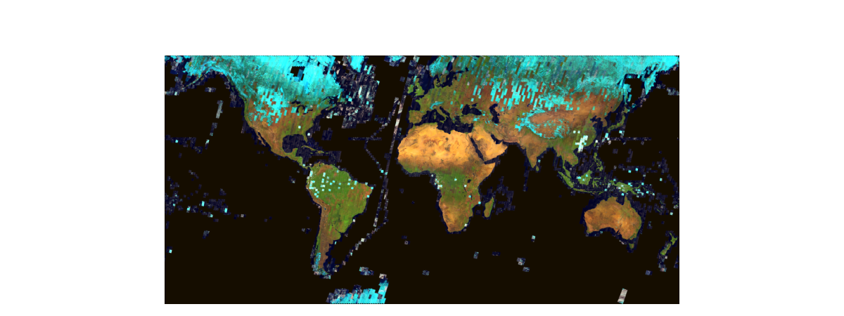
The code below cycles through and lists the Raster Functions published with the imglyr:
for fn in imglyr.properties['rasterFunctionInfos']:
    print (fn['name'])
Agriculture with DRA Bathymetric with DRA Color Infrared with DRA Geology with DRA Natural Color with DRA Short-wave Infrared with DRA Agriculture Bathymetric Color Infrared Geology Natural Color Short-wave Infrared NDVI Colorized Normalized Difference Moisture Index Colorized NDVI Raw NBR Raw Band 10 Surface Temperature in Fahrenheit Band 11 Surface Temperature in Fahrenheit Band 10 Surface Temperature in Celsius Band 11 Surface Temperature in Celsius None
Let us create a map widget and load this layer
map1 = gis.map("Marthas Basin, Montana")
map1
Note: Video above results after running the 3rd code cell below
map1.zoom = 12map1.content.add(imglyr)The utility of raster functions is better seen when we interactively cycle through these raster functions and apply them to the map. The code below cycles through the first 6 raster functions stored with the Imagery Layer and a small time delay to illustrate. The image processing occurs on-the-fly at display resolution to show how the layer can be visualized using these different raster functions published with the layer.
import time
from arcgis.raster.functions import apply

for fn in imglyr.properties['rasterFunctionInfos'][:6]:
    print(fn['name'])
    map1.content.add(apply(imglyr, fn['name']))
    time.sleep(4)
    map1.content.remove_all()
Agriculture with DRA Bathymetric with DRA Color Infrared with DRA Geology with DRA Natural Color with DRA Short-wave Infrared with DRA
Raster functions
Developers can create their own raster functions, by chaining different raster functions. For instance, the code below is doing an Extract Band and extracting out the [4,5,3] band combination, and applying a Stretch to get the land-water boundary visualization that makes it easy to see where land is and where water is. Its worth noting that the raster function is applied at display resolution and only for the visible extent using on the fly image processing.
from arcgis.raster.functions import stretch, extract_band

def process_bands(layer, bands):
    return stretch(extract_band(layer, bands),
                    stretch_type='percentclip', min_percent=0.1, max_percent=0.1, gamma=[1, 1, 1], dra=True)
Let us apply this raster function to the image layer to visualize the results.
map2 = gis.map("Marthas Basin, Montana")
map2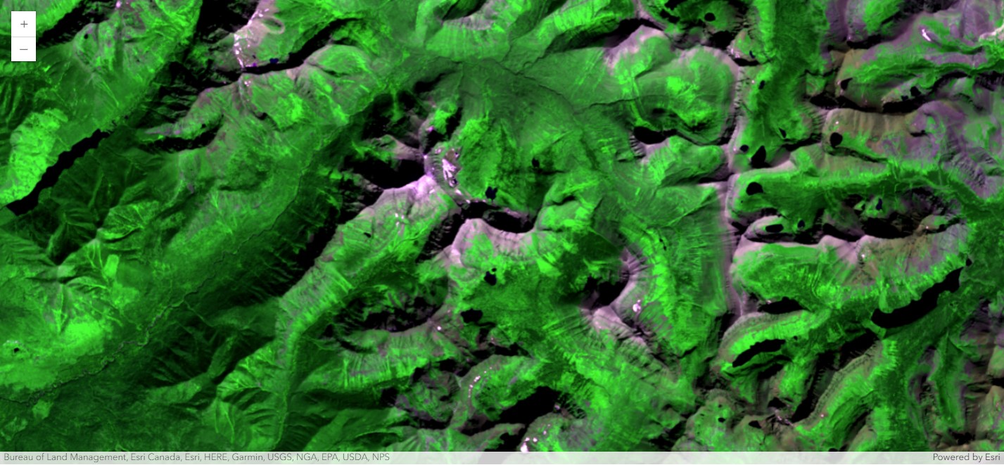
map2.content.add(process_bands(imglyr, [4, 5, 3]))
map2.zoom = 12
Creating a Raster Information Product using Landsat 8 imagery
This part of the notebook shows how Raster Analytics (in ArcGIS Enterprise 10.5) can be used to generate a raster information product, by applying the same raster function across the extent of an image service on the portal. The raster function is applied at source resolution and creates an Information Product, that can be used for further analysis and visualization.
montana_landsat = gis.content.get('b5625f3bad2f442a97fc8644d7d1e3ae')
montana_landsat
In the code below, we use extract and stretch the [7, 5, 2] band combination. This improves visibility of fire and burn scars by pushing further into the SWIR range of the electromagnetic spectrum, as there is less susceptibility to smoke and haze generated by a burning fire.
montana_lyr = montana_landsat.layers[0]fire_viz = process_bands(montana_lyr, [7, 5, 2])
fire_viz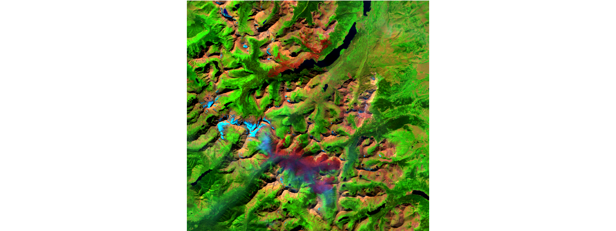
We can use the save method to apply the raster function across the entire extext of the input image layer at source resolution, and presist the result in an output image layer. This creates a raster product similar that can be used for further analysis and visualization.
arcgis.env.verbose = Truefrom datetime import datetime as dt
montana_fires_lyr = fire_viz.save('Montana_Burn_scars'+str(dt.now().microsecond))Submitted.
Executing...
Start Time: Tuesday, September 3, 2024 8:42:32 PM
Raster Analytics helper service: https://ip-172-31-20-195.us-east-2.compute.internal:6443/arcgis
Running on ArcGIS Image Server.
Image service {'name': 'Montana_Burn_scars883422', 'serviceUrl': 'https://pythonapi.playground.esri.com/ra/rest/services/Hosted/Montana_Burn_scars883422/ImageServer'} already existed.
Output item id is: 3043f5e015f845dd8c93848012770595
Output image service url is: https://ip-172-31-20-195.us-east-2.compute.internal:6443/arcgis/rest/services/Hosted/Montana_Burn_scars883422/ImageServer
Output cloud raster name is: Hosted_Montana_Burn_scars883422.crf
{"rasterFunction": "Stretch", "rasterFunctionArguments": {"Raster": {"rasterFunction": "ExtractBand", "rasterFunctionArguments": {"Raster": "https://pythonapi.playground.esri.com/ra/rest/services/ImgSrv_Landsat_Montana_2015/ImageServer?token=8pOUCPoDOhf2U9GlBUGwvCxaUFStvzgYFc2RNjmNPkAEuWGeGmAX7A1KqArjFO4vR_-tmF6cJXB-gdob2gGM3e6HzHL35zm9F5K3FhChSbP2hNT-X_Sm4ll3LEDV1BS9Hf33y2HLRPi-vC8UzpCRKlp2gkK7DVfkWx98FOpGDguWqt3mQCYzfOfKLKcnnEIci4VY2qJ5lwlRrMDDMJ0JL7Pduh6M7mmSmjVflH-R4dA.", "BandIDs": [6, 4, 1]}, "variableName": "Raster"}, "StretchType": 6, "DRA": true, "MinPercent": 0.1, "MaxPercent": 0.1, "Gamma": [1, 1, 1], "UseGamma": true}, "variableName": "Raster"}
Hosted_Montana_Burn_scars883422.crf
Updating service with data store URI.
Getting image service info...
Updating service: https://ip-172-31-20-195.us-east-2.compute.internal:6443/arcgis/admin/services/Hosted/Montana_Burn_scars883422.ImageServer/edit
Update item service: https://ip-172-31-20-195.us-east-2.compute.internal:6443/arcgis/admin/services/Hosted/Montana_Burn_scars883422.ImageServer successfully.
Portal item refreshed.
Succeeded at Tuesday, September 3, 2024 8:42:42 PM (Elapsed Time: 9.81 seconds)
GenerateRaster GP Job: j74760d92ca514bf59a855a3f1e78c885 finished successfully.
montana_fires_lyr
base_map = gis.map("Marthas Basin, Montana")

natural_color_map = gis.map("Marthas Basin, Montana")
natural_color_map.content.add(montana_landsat)

false_color_map = gis.map("Marthas Basin, Montana")
false_color_map.content.add(montana_fires_lyr)
base_map.zoom = 13
natural_color_map.zoom = 13
false_color_map.zoom = 13We can compare the natural color and false color images uaing a tabbed widget.
In the false color image the red and brownish pixels correspond to burn scars of the fire:
import ipywidgets as widgets

tab = widgets.Tab([base_map, natural_color_map, false_color_map])
tab.set_title(0, 'Basemap')
tab.set_title(1, 'Natural Color')
tab.set_title(2, 'False Color')
tab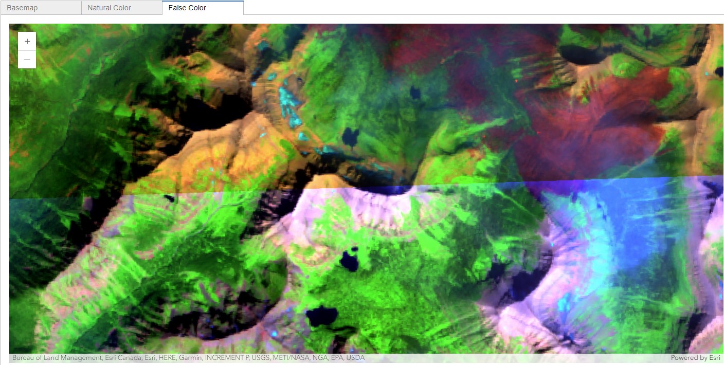
Thus using the same raster function, we were able to both visualize on the fly and derive a persisted image service using distributed raster analysis.