- 🔬 Data Science
- 🥠 Deep Learning and Object Detection
Introduction and objective
Deep Learning has achieved great success with state of the art results, but taking it to the field and solving real-world problems is still a challenge. Integration of the latest research in AI with ArcGIS opens up a world of opportunities. This notebook demonstrates an end-to-end deep learning workflow in using ArcGIS API for Python. The workflow consists of three major steps: (1) extract training data, (2) train a deep learning object detection model, (3) deploy the model for inference and create maps. To better illustrate this process, we choose detecting swmming pools in Redlands, CA using remote sensing imagery.

Part 1 - Export training data
To export training data, we need a labeled feature class that contains the bounding box for each object, and a raster layer that contains all the pixels and band information. In this swimming pool detection case, we have created feature class by hand labelling the bounding box of each swimming pool in Redlands using ArcGIS Pro and USA NAIP Imagery: Color Infrared as raster data.
from arcgis.gis import GIS
gis = GIS('home')
ent_gis = GIS('https://pythonapi.playground.esri.com/portal')
pool_bb = gis.content.get('0da0026a3a6d47dc8da0bcff6cf5bfb2')
pool_bbnaip_item = ent_gis.content.get('2f8f066d526e48afa9a942c675926785')
naip_itemWith the feature class and raster layer, we are now ready to export training data using the 'Export Training Data For Deep Learning' tool in arcgis Pro. In addtion to feature class, raster layer, and output folder, we also need to speficy a few other parameters such as tile size (size of the image chips), stride size (distance to move in the X when creating the next image chip), chip format (TIFF, PNG, or JPEG), metadata format (how we are going to store those bounding boxes).
Depending on the size of your data, tile and stride size, and computing resources, this opertation can take 15mins~2hrs in our experiment. Also, do not re-run it if you already run it once unless you would like to update the setting.

Part 2 - model training
If you've already done part 1, you should already have both the training chips and swimming pool labels. Please change the path to your own export training data folder that contains "images" and "labels" folder.
Necessary imports
import os
from pathlib import Path
from arcgis.gis import GIS
from arcgis.learn import prepare_data, AutoDL, ImageryModel
training_data = gis.content.get('73a29df69b344ce8b94fdb4c9df7103d')
training_datafilepath = training_data.download(file_name=training_data.name)import zipfile
with zipfile.ZipFile(filepath, 'r') as zip_ref:
zip_ref.extractall(Path(filepath).parent)data_path = Path(os.path.join(os.path.splitext(filepath)[0]))Prepare data that will be used for training
data = prepare_data(data_path,
                    batch_size=4,
                    chip_size=448,
                    class_mapping={'0': 'pool'})
data.classes
['background', 'pool']
Visualize training data
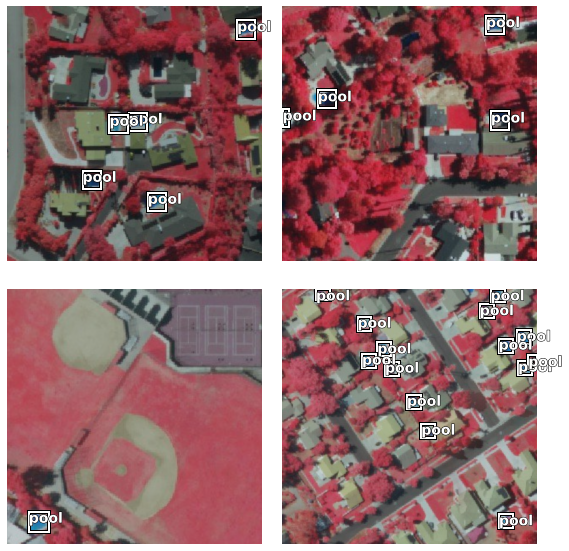
To get a sense of what the training data looks like, arcgis.learn.show_batch() method randomly picks a few training chips and visualize them.
%%time
data.show_batch()
Wall time: 2.97 s

Load model architecture
model = AutoDL(data, total_time_limit=2)Given time to process the dataset is: 2.0 hours Number of images that can be processed in the given time: 116 Time required to process the entire dataset of 1845 images is 31.6 hours
%%time
model.fit()
13-06-2022 15:32:37: Selected networks: SingleShotDetector RetinaNet FasterRCNN YOLOv3 atss carafe cascade_rcnn cascade_rpn dcn 13-06-2022 15:32:37: Current network - SingleShotDetector... 13-06-2022 15:32:37: Total time alloted to train the SingleShotDetector model is 0:06:11 13-06-2022 15:32:37: Maximum number of epochs will be 20 to train SingleShotDetector 13-06-2022 15:32:37: Initializing the SingleShotDetector network... 13-06-2022 15:32:39: SingleShotDetector initialized with resnet34 backbone 13-06-2022 15:32:39: Finding best learning rate for SingleShotDetector 13-06-2022 15:32:58: Best learning rate for SingleShotDetector with the selected data is 0.0030199517204020187 13-06-2022 15:32:58: Fitting SingleShotDetector 13-06-2022 15:35:58: Training completed 13-06-2022 15:35:58: Computing the network metrices 13-06-2022 15:36:02: Finished training SingleShotDetector. 13-06-2022 15:36:02: Exiting... 13-06-2022 15:36:02: Saving the model 13-06-2022 15:36:11: model saved at C:\Users\pri10421\AppData\Local\Temp\detecting_swimming_pools_using_satellite_image_and_deep_learning\models\AutoDL_SingleShotDetector_resnet34 13-06-2022 15:36:11: Current network - RetinaNet... 13-06-2022 15:36:11: Total time alloted to train the RetinaNet model is 0:25:19 13-06-2022 15:36:11: Maximum number of epochs will be 20 to train RetinaNet 13-06-2022 15:36:11: Initializing the RetinaNet network... 13-06-2022 15:36:15: RetinaNet initialized with resnet50 backbone 13-06-2022 15:36:15: Finding best learning rate for RetinaNet 13-06-2022 15:36:34: Best learning rate for RetinaNet with the selected data is 0.001 13-06-2022 15:36:34: Fitting RetinaNet 13-06-2022 15:38:39: Training completed 13-06-2022 15:38:39: Computing the network metrices 13-06-2022 15:38:48: Finished training RetinaNet. 13-06-2022 15:38:48: Exiting... 13-06-2022 15:38:48: Saving the model 13-06-2022 15:39:07: model saved at C:\Users\pri10421\AppData\Local\Temp\detecting_swimming_pools_using_satellite_image_and_deep_learning\models\AutoDL_RetinaNet_resnet50 13-06-2022 15:39:07: Current network - FasterRCNN... 13-06-2022 15:39:07: Total time alloted to train the FasterRCNN model is 0:25:19 13-06-2022 15:39:07: Maximum number of epochs will be 20 to train FasterRCNN 13-06-2022 15:39:07: Initializing the FasterRCNN network... 13-06-2022 15:39:08: FasterRCNN initialized with resnet50 backbone 13-06-2022 15:39:08: Finding best learning rate for FasterRCNN 13-06-2022 15:39:37: Best learning rate for FasterRCNN with the selected data is 0.00019054607179632462 13-06-2022 15:39:37: Fitting FasterRCNN 13-06-2022 15:42:58: Training completed 13-06-2022 15:42:58: Computing the network metrices 13-06-2022 15:43:07: Finished training FasterRCNN. 13-06-2022 15:43:07: Exiting... 13-06-2022 15:43:07: Saving the model 13-06-2022 15:43:25: model saved at C:\Users\pri10421\AppData\Local\Temp\detecting_swimming_pools_using_satellite_image_and_deep_learning\models\AutoDL_FasterRCNN_resnet50 13-06-2022 15:43:25: Current network - YOLOv3... 13-06-2022 15:43:25: Total time alloted to train the YOLOv3 model is 0:05:59 13-06-2022 15:43:25: Maximum number of epochs will be 20 to train YOLOv3 13-06-2022 15:43:25: Initializing the YOLOv3 network... 13-06-2022 15:43:26: YOLOv3 initialized with DarkNet53 backbone 13-06-2022 15:43:26: Finding best learning rate for YOLOv3 13-06-2022 15:43:50: Best learning rate for YOLOv3 with the selected data is 0.002511886431509582 13-06-2022 15:43:50: Fitting YOLOv3 13-06-2022 16:39:26: Training completed 13-06-2022 16:39:26: Computing the network metrices 13-06-2022 16:42:56: Finished training YOLOv3. 13-06-2022 16:42:56: Exiting... 13-06-2022 16:42:56: Saving the model 13-06-2022 16:46:53: model saved at C:\Users\pri10421\AppData\Local\Temp\detecting_swimming_pools_using_satellite_image_and_deep_learning\models\AutoDL_YOLOv3_DarkNet53 13-06-2022 16:46:53: deleting YOLOv3 with DarkNet53 13-06-2022 16:46:53: Current network - atss... 13-06-2022 16:46:53: Total time alloted to train the atss model is 0:06:22 13-06-2022 16:46:53: Maximum number of epochs will be 20 to train atss 13-06-2022 16:46:53: Initializing the atss network... 13-06-2022 16:47:08: atss initialized with resnet34 backbone 13-06-2022 16:47:08: Finding best learning rate for atss 13-06-2022 16:47:33: Best learning rate for atss with the selected data is 0.0005754399373371565 13-06-2022 16:47:33: Fitting atss 13-06-2022 16:52:07: Training completed 13-06-2022 16:52:07: Computing the network metrices 13-06-2022 16:52:13: Finished training atss. 13-06-2022 16:52:13: Exiting... 13-06-2022 16:52:13: Saving the model 13-06-2022 16:52:30: model saved at C:\Users\pri10421\AppData\Local\Temp\detecting_swimming_pools_using_satellite_image_and_deep_learning\models\AutoDL_atss_resnet34 13-06-2022 16:52:30: Current network - carafe... 13-06-2022 16:52:30: Total time alloted to train the carafe model is 0:13:32 13-06-2022 16:52:30: Maximum number of epochs will be 20 to train carafe 13-06-2022 16:52:30: Initializing the carafe network... 13-06-2022 16:52:31: carafe initialized with resnet34 backbone 13-06-2022 16:52:31: Finding best learning rate for carafe 13-06-2022 16:52:54: Best learning rate for carafe with the selected data is 4.365158322401661e-05 13-06-2022 16:52:54: Fitting carafe 13-06-2022 16:57:14: Training completed 13-06-2022 16:57:14: Computing the network metrices 13-06-2022 16:57:20: Finished training carafe. 13-06-2022 16:57:20: Exiting... 13-06-2022 16:57:20: Saving the model 13-06-2022 16:57:38: model saved at C:\Users\pri10421\AppData\Local\Temp\detecting_swimming_pools_using_satellite_image_and_deep_learning\models\AutoDL_carafe_resnet34 13-06-2022 16:57:38: deleting carafe with resnet34 13-06-2022 16:57:38: Current network - cascade_rcnn... 13-06-2022 16:57:38: Total time alloted to train the cascade_rcnn model is 0:02:42 13-06-2022 16:57:38: Maximum number of epochs will be 20 to train cascade_rcnn 13-06-2022 16:57:38: Initializing the cascade_rcnn network... 13-06-2022 16:57:40: cascade_rcnn initialized with resnet34 backbone 13-06-2022 16:57:40: Finding best learning rate for cascade_rcnn 13-06-2022 16:58:17: Best learning rate for cascade_rcnn with the selected data is 2.0892961308540385e-05 13-06-2022 16:58:17: Fitting cascade_rcnn 13-06-2022 17:06:54: Training completed 13-06-2022 17:06:54: Computing the network metrices 13-06-2022 17:07:05: Finished training cascade_rcnn. 13-06-2022 17:07:05: Exiting... 13-06-2022 17:07:05: Saving the model 13-06-2022 17:07:42: model saved at C:\Users\pri10421\AppData\Local\Temp\detecting_swimming_pools_using_satellite_image_and_deep_learning\models\AutoDL_cascade_rcnn_resnet34 13-06-2022 17:07:42: deleting cascade_rcnn with resnet34 13-06-2022 17:07:42: Current network - cascade_rpn... 13-06-2022 17:07:42: Total time alloted to train the cascade_rpn model is 0:16:14 13-06-2022 17:07:42: Maximum number of epochs will be 20 to train cascade_rpn 13-06-2022 17:07:42: Initializing the cascade_rpn network... 13-06-2022 17:07:42: cascade_rpn initialized with resnet34 backbone 13-06-2022 17:07:42: Finding best learning rate for cascade_rpn 13-06-2022 17:08:07: Best learning rate for cascade_rpn with the selected data is 7.585775750291836e-05 13-06-2022 17:08:07: Fitting cascade_rpn 13-06-2022 17:14:46: Training completed 13-06-2022 17:14:46: Computing the network metrices 13-06-2022 17:14:54: Finished training cascade_rpn. 13-06-2022 17:14:54: Exiting... 13-06-2022 17:14:54: Saving the model 13-06-2022 17:15:11: model saved at C:\Users\pri10421\AppData\Local\Temp\detecting_swimming_pools_using_satellite_image_and_deep_learning\models\AutoDL_cascade_rpn_resnet34 13-06-2022 17:15:11: deleting cascade_rpn with resnet34 13-06-2022 17:15:11: Current network - dcn... 13-06-2022 17:15:11: Total time alloted to train the dcn model is 0:16:14 13-06-2022 17:15:11: Maximum number of epochs will be 20 to train dcn 13-06-2022 17:15:11: Initializing the dcn network... 13-06-2022 17:15:12: dcn initialized with resnet34 backbone 13-06-2022 17:15:12: Finding best learning rate for dcn 13-06-2022 17:15:40: Best learning rate for dcn with the selected data is 2.0892961308540385e-05 13-06-2022 17:15:40: Fitting dcn 13-06-2022 17:23:04: Training completed 13-06-2022 17:23:04: Computing the network metrices
13-06-2022 17:23:12: Finished training dcn.
13-06-2022 17:23:12: Exiting...
13-06-2022 17:23:12: Saving the model
Computing model metrics...
13-06-2022 17:23:37: model saved at C:\Users\pri10421\AppData\Local\Temp\detecting_swimming_pools_using_satellite_image_and_deep_learning\models\AutoDL_dcn_resnet34
13-06-2022 17:23:37: deleting dcn with resnet34
13-06-2022 17:23:37: Collating and evaluating model performances...
13-06-2022 17:23:37: Exiting...
Wall time: 1h 50min 59s
score = model.average_precision_score()
score.sort_values(by='pool', ascending=False)| Model | pool | |
|---|---|---|
| 0 | atss | 0.545365 |
| 0 | carafe | 0.542435 |
| 0 | dcn | 0.536729 |
| 0 | cascade_rcnn | 0.536235 |
| 0 | FasterRCNN | 0.519933 |
| 0 | cascade_rpn | 0.298964 |
| 0 | RetinaNet | 0.268603 |
| 0 | SingleShotDetector | 0.054507 |
| 0 | YOLOv3 | 0.011685 |
from arcgis.learn import ImageryModelmodel = ImageryModel()model.load(r'C:\Users\pri10421\AppData\Local\Temp\detecting_swimming_pools_using_satellite_image_and_deep_learning\models\AutoDL_atss_resnet34\AutoDL_atss_resnet34.emd',
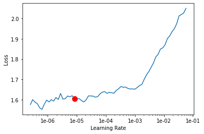
data)lr = model.lr_find()
Train the model
model.fit(epochs=10, lr=lr)| epoch | train_loss | valid_loss | time |
|---|---|---|---|
| 0 | 1.609834 | 1.590176 | 02:03 |
| 1 | 1.605651 | 1.568000 | 02:05 |
| 2 | 1.605779 | 1.546265 | 02:05 |
| 3 | 1.556396 | 1.564944 | 02:05 |
| 4 | 1.550402 | 1.529054 | 02:04 |
| 5 | 1.536427 | 1.531565 | 02:04 |
| 6 | 1.499966 | 1.520815 | 02:04 |
| 7 | 1.543200 | 1.512366 | 02:03 |
| 8 | 1.513313 | 1.504317 | 02:04 |
| 9 | 1.541665 | 1.507654 | 02:04 |
model.average_precision_score(){'pool': 0.5137461662102243}model.fit(epochs=10)| epoch | train_loss | valid_loss | time |
|---|---|---|---|
| 0 | 1.504260 | 1.501823 | 02:02 |
| 1 | 1.519276 | 1.513599 | 02:03 |
| 2 | 1.559772 | 1.526369 | 02:04 |
| 3 | 1.510672 | 1.485849 | 02:03 |
| 4 | 1.563332 | 1.506348 | 02:04 |
| 5 | 1.521287 | 1.514715 | 02:04 |
| 6 | 1.521208 | 1.519161 | 02:04 |
| 7 | 1.502555 | 1.497568 | 02:06 |
| 8 | 1.529561 | 1.501051 | 02:04 |
| 9 | 1.505702 | 1.497763 | 02:04 |
model.average_precision_score(){'pool': 0.5561870892632037}Detect and visualize swimming pools in validation set
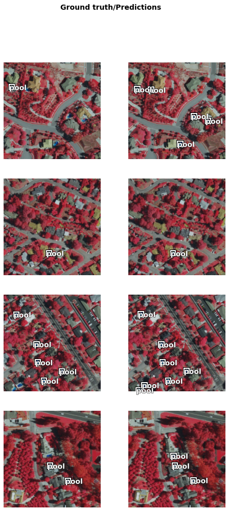
Now we have the model, let's look at how the model performs. Here we plot out 5 rows of images and a threshold of 0.2. Threshold is a measure of probablity that a swimming pool exists. Higher value meas more confidence.
model.show_results(thresh=0.2)
As we can see, with only 20 epochs, we are already seeing reasonable results. Further improvment can be acheived through more sophisticated hyperparameter tuning. Let's save the model for further training or inference later. The model should be saved into a models folder in your folder. By default, it will be saved into your data_path that you specified in the very beginning of this notebook.
model.save('PoolDetection_USA_20')Computing model metrics...
Part 3 - Model inference
To test our model, let's get a raster image with some swimming pools.

Visualize detected pools on map
predicted_result = gis.content.get('793d2060d14746d19ee4c45d3eda7724')
predicted_resultresult_map = gis.map('Redlands, CA')
result_map.add_layer(naip_item.layers[0])
result_map.add_layer(predicted_result.layers[0])
result_map = {'spatialReference': {'latestWkid': 3857, 'wkid': 102100},
'xmin': -13044535.370791622,'ymin': 4045062.583115232,
'xmax': -13042184.932171792,'ymax': 4046018.045968822}
result_map
Conclusion
In thise notebook, we have covered a lot of ground. In part 1, we discussed how to export training data for deep learning using ArcGIS Pro, we demonstrated how to prepare the input data, train a object detection model, visualize the results, as well as apply the model to an unseen image using the Detect Objects Using Deep Learning tool in ArcGIS Pro.
References
[1] Wei Liu, Dragomir Anguelov, Dumitru Erhan, Christian Szegedy, Scott Reed, Cheng-Yang Fu: “SSD: Single Shot MultiBox Detector”, 2015; arXiv:1512.02325.


