- 🔬 Data Science
- 🥠 Deep Learning and Segmentation
Introduction
With the change in global climate, glaciers all over the world are experiencing an increasing mass loss, resulting in changing calving fronts. This calving front delineation is important for monitoring the rate of glacial mass loss. Currently, most calving front delineation is done manually, resulting in excessive time consumption and under-utilization of satellite imagery.
Extracting calving fronts from satellite images of marine-terminating glaciers is a two-step process. The first step involves segmenting the front using different segmentation techniques, and the second step involves post-processing mechanisms to extract the terminus line. This notebook presents the use of an HRNet model from the arcgis.learn module to accomplish the first task of segmenting calving fronts. We have used data provided in the CALFIN repository. The training data includes 1600+ Greenlandic glaciers and 200+ Antarctic glaciers/ice shelves images from Landsat (optical) and Sentinel-1 (SAR) satellites.
Necessary imports
import os
import glob
import zipfile
from pathlib import Path

from arcgis.gis import GIS
from arcgis.learn import MMSegmentation, prepare_data
Connect to your GIS
# Connect to GIS
gis = GIS("home")
Download training data
training_data = gis.content.get('cc750295180a487aa7af67a67cadff78')
training_data
The data size is approximately 6.5 GBs and may take some time to download.
filepath = training_data.download(file_name=training_data.name)with zipfile.ZipFile(filepath, 'r') as zip_ref:
zip_ref.extractall(Path(filepath).parent)output_path = os.path.join(os.path.splitext(filepath)[0])output_path = glob.glob(output_path)Train the model
arcgis.learn provides an HRNet model through the integration of the MMSegmentation class. For more in-depth information on MMSegmentation, see this guide - Using MMSegmentation with arcgis.learn.
Prepare data
Next, we will specify the path to our training data and a few hyperparameters.
path: path of the folder/list of folders containing the training data.batch_size: The number of images your model will train on for each step of an epoch. This will directly depend on the memory of your graphics card.
data = prepare_data(path=output_path, dataset_type='Classified_Tiles', batch_size=24)Visualize training data
To get a sense of what the training data looks like, the arcgis.learn.show_batch() method will randomly select training chips and visualizes them.
rows: Number of rows to visualize
data.show_batch(5, alpha=0.7)
Load model architecture
model = MMSegmentation(data, 'hrnet')Find an optimal learning rate
Learning rate is one of the most important hyperparameters in model training. ArcGIS API for Python provides a learning rate finder that automatically chooses the optimal learning rate for you.
lr = model.lr_find()
Fit the model
Next, we will train the model for a few epochs with the learning rate found in the previous step. For the sake of time, we will start with 30 epochs.
model.fit(30, lr)| epoch | train_loss | valid_loss | accuracy | dice | time |
|---|---|---|---|---|---|
| 0 | 0.610420 | 0.560476 | 0.724492 | 0.302636 | 03:44 |
| 1 | 0.557933 | 0.496885 | 0.757505 | 0.353984 | 03:45 |
| 2 | 0.489416 | 0.445652 | 0.789769 | 0.501799 | 03:46 |
| 3 | 0.447124 | 0.496963 | 0.756810 | 0.567582 | 03:47 |
| 4 | 0.427683 | 0.378213 | 0.833140 | 0.528805 | 03:51 |
| 5 | 0.399223 | 0.365552 | 0.842118 | 0.531487 | 03:53 |
| 6 | 0.381643 | 0.401336 | 0.811905 | 0.534826 | 03:54 |
| 7 | 0.378017 | 0.605405 | 0.757742 | 0.177460 | 03:52 |
| 8 | 0.367449 | 0.422544 | 0.815683 | 0.612659 | 03:50 |
| 9 | 0.358794 | 0.401540 | 0.804915 | 0.574714 | 03:50 |
| 10 | 0.342343 | 0.404026 | 0.843801 | 0.464923 | 03:52 |
| 11 | 0.344887 | 0.333360 | 0.859139 | 0.634893 | 03:48 |
| 12 | 0.334531 | 0.433300 | 0.843079 | 0.530823 | 03:50 |
| 13 | 0.312203 | 0.342381 | 0.851830 | 0.672622 | 03:47 |
| 14 | 0.318387 | 0.365772 | 0.850246 | 0.479703 | 03:44 |
| 15 | 0.304587 | 0.272239 | 0.889210 | 0.672367 | 03:44 |
| 16 | 0.299469 | 0.255955 | 0.889639 | 0.727745 | 03:43 |
| 17 | 0.290696 | 0.281389 | 0.882833 | 0.684749 | 03:43 |
| 18 | 0.279878 | 0.255700 | 0.896031 | 0.719328 | 03:43 |
| 19 | 0.272493 | 0.221865 | 0.912843 | 0.722819 | 03:43 |
| 20 | 0.254924 | 0.228055 | 0.907706 | 0.736925 | 03:45 |
| 21 | 0.253474 | 0.230905 | 0.901044 | 0.754613 | 03:47 |
| 22 | 0.248331 | 0.214303 | 0.918499 | 0.752050 | 03:49 |
| 23 | 0.234423 | 0.199226 | 0.926057 | 0.770178 | 03:48 |
| 24 | 0.238598 | 0.198984 | 0.923163 | 0.778105 | 03:49 |
| 25 | 0.228168 | 0.200712 | 0.920581 | 0.771879 | 03:48 |
| 26 | 0.235029 | 0.190604 | 0.925844 | 0.777296 | 03:47 |
| 27 | 0.221403 | 0.194644 | 0.925728 | 0.784709 | 03:47 |
| 28 | 0.230099 | 0.192264 | 0.927934 | 0.786932 | 03:49 |
| 29 | 0.219289 | 0.190728 | 0.926994 | 0.781577 | 03:46 |
As we can see, the training and validation losses are continuing to decrease, indicating that the model is still learning. This suggests that there is more room for training, and as such, we chose to train the model for a total of 170 epochs to achieve better results.
Visualize results in validation set
It is a good practice to see the results of the model viz-a-viz ground truth. The code below picks random samples and visualizes the ground truth and model predictions side by side. This enables us to preview the results of the model we trained for 170 epochs within the notebook.
model.show_results(5, thresh=0.1, aplha=0.1)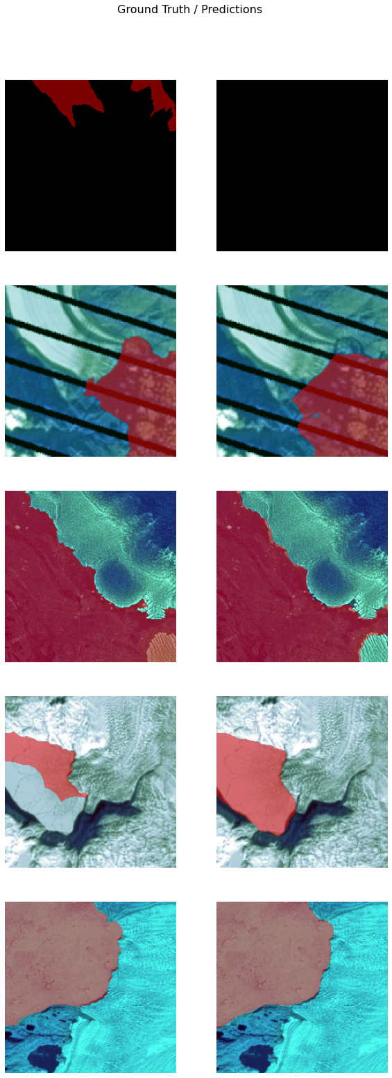
Accuracy assessment
arcgis.learn provides the mIOU() method that computes the mean IOU (Intersection over Union) on the validation set for each class.
model.mIOU(){'0': 0.9026798871510977, 'Masked': 0.7716700616812664}model.per_class_metrics()| NoData | Masked | |
|---|---|---|
| precision | 0.937634 | 0.899602 |
| recall | 0.960069 | 0.848553 |
| f1 | 0.948719 | 0.873332 |
Save the model
We will save the model which we trained as a 'Deep Learning Package' ('.dlpk' format). The Deep Learning package is the standard format used to deploy deep learning models on the ArcGIS platform.
We will use the save() method to save the trained model. By default, it will be saved to the 'models' sub-folder within our training data folder.
model.save("Glaciertips_hrnet_30e", publish=True)Published DLPK Item Id: 2f4454094f974f74b1e67432bcaf564d
WindowsPath('D:/Glacier Tips/data/data for notebook/glacial_terminus_point_segmentation/models/Glaciertips_hrnet_30e')The saved model in this notebook can be downloaded from this link.
Model inference
In this step, we will generate a classified raster using the 'Classify Pixels Using Deep Learning' tool available in both ArcGIS Pro and ArcGIS Enterprise.
Input Raster: The raster layer you want to classify.Model Definition: Located inside the saved model in the 'models' folder in '.emd' format.Padding: The 'Input Raster' is tiled, and the deep learning model classifies each individual tile separately before producing the final 'Output Classified Raster'. This may lead to unwanted artifacts along the edges of each tile, as the model has little context to predict accurately. Padding allows us to supply extra information along the tile edges, thus helping the model to make better predictions.Cell Size: Should be close to the size used to train the model.Processor Type: Allows you to control whether the system's 'GPU' or 'CPU' will be used to classify pixels. By default, 'GPU' will be used if available.

It is advised to zoom in to the right extent of the area of interest in order to avoid/reduce noise from the results as the model is not trained to be generalized to work across the globe.
Results
The gif below was achieved with the model trained in this notebook and visualizes the segmented calving front for Rink Isbrae, a major West Greenland outlet glacier.

Conclusion
In this notebook, we have demonstrated how to use models supported by the MMSegmentation class in arcgis.learn to perform segmentation tasks. We trained an HRNet model to segment calving fronts for the Risk Isbrae glacier. With this trained model, this segmentation task can now be performed in regular intervals to monitor glacial mass loss.