These tools help you identify, quantify, and visualize spatial patterns in your data.
calculate_density takes known quantities of some phenomenon and spreads these quantities across the map. find_hot_spots identifies statistically significant clustering in the spatial pattern of your data.
calculate_density
-
arcgis.geoanalytics.analyze_patterns.calculate_density(input_layer, fields=None, weight='Uniform', bin_type='Square', bin_size=None, bin_size_unit=None, time_step_interval=None, time_step_interval_unit=None, time_step_repeat_interval=None, time_step_repeat_interval_unit=None, time_step_reference=None, radius=None, radius_unit=None, area_units='SquareKilometers', output_name=None, gis=None, context=None, future=False)¶ 
The
calculate_densitytool creates a density map from point features by spreading known quantities of some phenomenon (represented as attributes of the points) across the map. The result is a layer of areas classified from least dense to most dense.For point input, each point should represent the location of some event or incident, and the result layer represents a count of the incident per unit area. A higher density value in a new location means that there are more points near that location. In many cases, the result layer can be interpreted as a risk surface for future events. For example, if the input points represent locations of lightning strikes, the result layer can be interpreted as a risk surface for future lightning strikes.
Other use cases of this tool include the following:
Creating crime density maps to help police departments properly allocate resources to high crime areas.
Calculating densities of hospitals within a county. The result layer will show areas with high and low accessibility to ospitals, and this information can be used to decide where new hospitals should be built.
Identifying areas that are at high risk of forest fires based on historical locations of forest fires.
Locating communities that are far from major highways in order to plan where new roads should be constructed.
Parameter
Description
input_layer
Required point feature layer. The point layer on which the density will be calculated.
See Feature Input.
Note
Analysis using bins requires a projected coordinate system. When aggregating layers into bins, the input layer or processing extent (
processSR) must have a projected coordinate system. At 10.5.1, 10.6, and 10.6.1, if a projected coordinate system is not specified when running analysis, the World Cylindrical Equal Area (WKID 54034) projection will be used. At 10.7 or later, if a projected coordinate system is not specified when running analysis, a projection will be picked based on the extent of the data.fields
Optional string. Provides one or more field specifying the number of incidents at each location. You can calculate the density on multiple fields, and the count of points will always have the density calculated.
weight
Required string. The type of weighting applied to the density calculation. There are two options:
Uniform- Calculates a magnitude-per-area. This is the default.Kernel- Applies a kernel function to fit a smooth tapered surface to each point.
The default value is “Uniform”.
bin_type
Required string. The type of bin used to calculate density.
Note
Analysis using
SquareorHexagonbins requires a projected coordinate system. When aggregating layers into bins, the input layer or processing extent (processSR) must have a projected coordinate system. At 10.5.1, 10.6, and 10.6.1, if a projected coordinate system is not specified when running analysis, the World Cylindrical Equal Area (WKID 54034) projection will be used. At 10.7 or later, if a projected coordinate system is not specified when running analysis, a projection will be picked based on the extent of the data.Choice list:
HexagonSquare
bin_size
Required float. The distance for the bins that the
input_layerwill be analyzed using. When generating bins, for Square, the number and units specified determine the height and length of the square. ForHexagon, the number and units specified determine the distance between parallel sides.bin_size_unit
Required string. The distance unit for the bins for which the density will be calculated. The linear unit to be used with the value specified in
bin_size.The default is ‘Meters’.
time_step_interval
Optional integer. A numeric value that specifies duration of the time step interval. This option is only available if the input points are time-enabled and represent an instant in time.
The default value is ‘None’.
time_step_interval_unit
Optional string. A string that specifies units of the time step interval. This option is only available if the input points are time-enabled and represent an instant in time.
Choice list:
MillisecondsSecondsMinutesHoursDaysWeeksMonthsYears
The default value is ‘None’.
time_step_repeat_interval
Optional integer. A numeric value that specifies how often the time step repeat occurs. This option is only available if the input points are time-enabled and of time type instant.
time_step_repeat_interval_unit
Optional string. A string that specifies the temporal unit of the step repeat. This option is only available if the input points are time-enabled and of time type instant.
Choice list:
YearsMonthsWeeksDaysHoursMinutesSecondsMilliseconds
The default value is ‘None’.
time_step_reference
Optional datetime. A date that specifies the reference time to align the time slices to, represented in milliseconds from epoch. If time_step_reference is set to ‘None’, time stepping will align to January 1st, 1970 (datetime(1970, 1, 1)). This option is only available if the input points are time-enabled and of time type instant.
The default value is ‘None’.
radius
Required integer. The size of the neighborhood within which to calculate the density. The radius size must be larger than the
bin_size.radius_unit
Required string. The distance unit for the radius defining the neighborhood for which the density will be calculated. The linear unit to be used with the value specified in
bin_size.Choice list:
FeetYardsMilesMetersKilometersNauticalMiles
The default value is ‘Meters’.
area_units
Optional string. The desired output units of the density values. If density values are very small, you can increase the size of the area units (for example, square meters to square kilometers) to return larger values. This value only scales the result. Possible area units are:
Choice list:
SquareMetersSquareKilometersHectaresSquareFeetSquareYardsSquareMilesAcres
The default value is
SquareKilometers.output_name
Optional string. The method will create a feature service of the results. You define the name of the service.
gis
Optional, the GIS on which this tool runs. If not specified, the active GIS is used.
context
Optional dict. The context parameter contains additional settings that affect task execution. For this task, there are four settings (keys in the dictionary):
Extent (
extent) - A bounding box that defines the analysis area. Only those features that intersect the bounding box will be analyzed.Processing spatial reference (
processSR) - The features will be projected into this coordinate system for analysis.Output spatial reference (
outSR) - The features will be projected into this coordinate system after the analysis to be saved. The output spatial reference for the spatiotemporal big data store is always WGS84.Data store (
dataStore) - Results will be saved to the specified data store. For ArcGIS Enterprise, the default is the spatiotemporal big data store.
future
Optional boolean. If True, a future object will be returned and the process will not wait for the task to complete. The default is False, which means wait for results.
- Returns
result_layer : Output Features as
FeatureLayer.
# Usage Example: Aggregate the number of Hurricanes within 1 meter to calculate density of Hurricane damage.

cal_den_result = calculate_density(input_layer=hurricane_lyr,
                                   fields='Damage',
                                   weight='Uniform',
                                   bin_type='Square',
                                   bin_size=1,
                                   bin_size_unit="Meters",
                                   radius=2,
                                   radius_unit="Yards")
create_space_time_cube
-
arcgis.geoanalytics.analyze_patterns.create_space_time_cube(point_layer, bin_size, bin_size_unit, time_step_interval, time_step_interval_unit, time_step_alignment=None, time_step_reference=None, summary_fields=None, output_name=None, context=None, gis=None, future=False)¶ 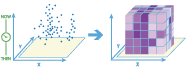
create_space_time_cubeworks with a layer of point features that are time enabled. It aggregates the data into a three-dimensional cube of space-time bins. When determining the point in a space-time bin relationship, statistics about all points in the space-time bins are calculated and assigned to the bins. The most basic statistic is the number of points within the bins, but you can calculate other statistics as well. For example, suppose you have point features of crimes in a city, and you want to summarize the number of crimes in both space and time. You can calculate the space-time cube for the dataset, and use the cube to further analyze trends such as emerging hot and cold spots.Parameter
Description
point_layer
Required point feature layer. The point features that will be aggregated into the bins specified in geographical size by the
bin_sizeandbin_size_unitparameters and temporal size by thetime_step_intervalandtime_step_interval_unitparameters. See Feature Input.Note
The
input_layermust have a minimum of 60 features.Note
Analysis using bins requires a projected coordinate system. When aggregating layers into bins, the input layer or processing extent (
processSR) must have a projected coordinate system. At 10.5.1, 10.6, and 10.6.1, if a projected coordinate system is not specified when running analysis, the World Cylindrical Equal Area (WKID 54034) projection will be used. At 10.7 or later, if a projected coordinate system is not specified when running analysis, a projection will be picked based on the extent of the data.bin_size
Required float. The distance for the bins into which
point_layerwill be aggregated.bin_size_unit
Required string. The distance unit for the bins into which
point_layerwill be aggregated.Choice list:
FeetYardsMilesMetersKilometersNauticalMiles
time_step_interval
Required integer. A numeric value that specifies the duration of the time bin.
Note
A
create_space_time_cubemust have at least 10 time slices.time_step_interval_unit
Required string. A numeric value that specifies the duration unit of the time bin.
Choice list:
YearsMonthsWeeksDaysHoursMinutesSecondsMilliseconds
time_step_alignment
Optional string. Defines how aggregation will occur based on a given timeInterval. Options are as follows:
Choice list:
StartTime- Time is aligned to the first feature in timeEndTime- Time is aligned to the last feature in timeReferenceTime- Time is aligned a specified time
time_step_reference (Required if
time_step_alignmentis ReferenceTime)Optional datetime. A date that specifies the reference time to align the time bins to if ReferenceTime is specified in
time_step_alignment.summary_fields
Optional list of dictiaries defining field names, statistical summary types, and the fill option for empty values that you want to calculate for all points within each space-time bin. Note that the count of points within each bin is always returned. By default, all statistics are returned.
Format:
[{"statisticType": "statistic type",
  "onStatisticField": "field name",
  "fillType": "fill type"},
 {"statisticType": "statistic type",
  "onStatisticField": "fieldName2",
  "fillType": "fill type"}]
statisticTypeis one of the following for numeric fields:Sum- Adds the total value of all the points in each polygon.Mean- Calculates the average of all the points in each polygon.Min- Finds the smallest value of all the points in each polygon.Max- Finds the largest value of all the points in each polygon.Stddev- Finds the standard deviation of all the points in each polygon.
statisticTypeis the following for string fields:Count- Totals the number of strings for all the points in each polygon.
onStatisticFieldis the name of fields in the input point layer.fillTypeis one of the following:zeros- Fills missing values with zeros. This is most appropriate for fields representing counts.spatialNeighbors- Fills missing values by averaging the spatial neighbors. Neighbors are determined by a second degree queens contiguity.spaceTimeNeighbors- Fills missing values by averaging the space-time neighbors. Neighbors are determined by a second degree queens contiguity in both space and time.temporalTrend- Interpolates values using a univariate spline.
output_name
Required string. The task will create a space time cube (netCDF) of the results. You define the name of the space time cube.
context
Optional string. Context contains additional settings that affect task execution. For this task, there are two settings:
extent- A bounding box that defines the analysis area. Only those features that intersect the bounding box will be analyzed.processSR- The features will be projected into this coordinate system for analysis.
gis
Optional, the
GISon which this tool runs. If not specified, the active GIS is used.future
Optional boolean. If
true, a future object will be returned and the process will not wait for the task to complete. The default isfalse, which means wait for results.- Returns
Dict with url containing the path to Output Space Time Cube (netCDF) dataFile. When you browse to the output url, your netCDF will automatically download to your local machine.
# Usage Example: To aggregate Chicago homicides date layer into 3-dimensional cubes of 5 miles bin.
create_space_time_cube(point_layer=lyr,
                       bin_size=5,
                       bin_size_unit="Miles",
                       time_step_interval=1,
                       time_step_interval_unit="Days",
                       time_step_alignment='StartTime',
                       time_step_reference=datetime(1995, 10, 4),
                       summary_fields=[{"statisticType": "Mean", "onStatisticField" : "Beat", "fillType" : "temporalTrend" }],
                       output_name="spacecube")
find_hot_spots
-
arcgis.geoanalytics.analyze_patterns.find_hot_spots(point_layer, bin_size=5, bin_size_unit='Miles', neighborhood_distance=5, neighborhood_distance_unit='Miles', time_step_interval=None, time_step_interval_unit=None, time_step_alignment=None, time_step_reference=None, output_name=None, gis=None, context=None, future=False)¶ 
The
find_hot_spotstool analyzes point data (such as crime incidents, traffic accidents, trees, and so on) or field values associated with points. It finds statistically significant spatial clusters of high incidents (hot spots) and low incidents (cold spots). Hot spots are locations with lots of points and cold spots are locations with very few points.The result map layer shows hot spots in red and cold spots in blue. The darkest red features indicate the strongest clustering of point densities; you can be 99 percent confident that the clustering associated with these features could not be the result of random chance. Similarly, the darkest blue features are associated with the strongest spatial clustering of the lowest point densities. Features that are beige are not part of a statistically significant cluster; the spatial pattern associated with these features could very likely be the result of random processes and random chance.
Parameter
Description
point_layer
Required feature layer. The point feature layer for which hot spots will be calculated. See Feature Input.
Note
Analysis using bins requires a projected coordinate system. When aggregating layers into bins, the input layer or processing extent (
processSR) must have a projected coordinate system. At 10.5.1, 10.6, and 10.6.1, if a projected coordinate system is not specified when running analysis, the World Cylindrical Equal Area (WKID 54034) projection will be used. At 10.7 or later, if a projected coordinate system is not specified when running analysis, a projection will be picked based on the extent of the data.bin_size
Optional float. The distance for the square bins the
point_layerwill be aggregated into.bin_size_unit
Optional string. The distance unit for the bins with which hot spots will be calculated. The linear unit to be used with the value specified in
bin_size. When generating bins the number and units specified determine the height and length of the square.Choice list:
FeetYardsMilesMetersKilometersNauticalMiles
The default value is
Miles.neighborhood_distance
Optional float. The size of the neighborhood within which to calculate the hot spots. The radius size must be larger than
bin_size.neighborhood_distance_unit
Optional string. The distance unit for the radius defining the neighborhood where the hot spots will be calculated. The linear unit to be used with the value specified in
bin_size.Choice list:
FeetYardsMilesMetersKilometersNauticalMiles
The default value is
Miles.time_step_interval
Optional integer. A numeric value that specifies duration of the time step interval. This option is only available if the input points are time-enabled and represent an instant in time.
time_step_interval_unit
Optional string. A string that specifies units of the time step interval. This option is only available if the input points are time-enabled and represent an instant in time.
Choice list:
YearsMonthsWeeksDaysHoursMinutesSecondsMilliseconds
time_step_alignment
Optional string. Defines how aggregation will occur based on a given
time_step_interval. Options are as follows:Choice list:
StartTime- Time is aligned to the first feature in time.EndTime- Time is aligned to the last feature in time.ReferenceTime- Time is aligned a specified time intime_step_reference.
time_step_reference (Required if
time_step_alignmentis ReferenceTime)Optional datetime. A date that specifies the reference time to align the time slices to. This option is only available if the input points are time-enabled and of time type instant.
output_name
Optional string. The task will create a feature service of the results. You define the name of the service.
context
Optional string. Context contains additional settings that affect task execution. For this task, there are four settings:
extent- a bounding box that defines the analysis area. Only those features that intersect the bounding box will be analyzed.processSRThe features will be projected into this coordinate system for analysis.outSR- the features will be projected into this coordinate system after the analysis to be saved.The output spatial reference for the spatiotemporal big data store is always WGS84.dataStore- Results will be saved to the specified data store. The default is the spatiotemporal big data store.
gis
Optional, the
GISon which this tool runs. If not specified, the active GIS is used.future
Optional boolean. If
true, a future object will be returned and the process will not wait for the task to complete. The default isfalse, which means wait for results.- Returns
Output Features as a
FeatureLayerCollectionitem
# Usage Example: To find significantly hot or cold spots of fire incidents.
find_hot_spots(point_layer=fire,
               bin_size=5,
               bin_size_unit='Miles',
               neighborhood_distance=5,
               neighborhood_distance_unit='Miles',
               time_step_interval=1,
               time_step_interval_unit='Years',
               time_step_alignment='StartTime',
               time_step_reference=None,
               output_name='find hot spots',
               context={'extent': {'xmin': -122.68,
                                   'ymin': 45.5,
                                   'xmax': -122.45,
                                   'ymax': 45.6
                                   'spatialReference': {'wkid': 4326}},
                        'outSR':{'wkid': 3857}}
              )
find_point_clusters
-
arcgis.geoanalytics.analyze_patterns.find_point_clusters(input_layer, method, min_feature_clusters, search_distance=None, distance_unit=None, output_name=None, gis=None, context=None, future=False, time_method=None, search_duration=None, duration_unit=None)¶ This tool extracts clusters from your input point features and identifies any surrounding noise.
For example, a nongovernmental organization is studying a particular pest-borne disease. It has a point dataset representing households in a study area, some of which are infested, and some of which are not. By using the Find Point Clusters tool, an analyst can determine clusters of infested households to help pinpoint an area to begin treatment and extermination of pests.
Parameter
Description
input_layer
The point features for which clusters will be found.
See Feature Input for options.
method
required String. The algorithm used for cluster analysis. This parameter must be specified as one of:
DBSCANHDBSCAN
min_feature_clusters
optional Integer. Minimum number of points to consider a cluster.
search_distance
optional Float. The distance to search between points to form a cluster.
Note
This is required for DBSCAN.
distance_unit
optional String. The search_distance units.
output_name
optional String. The task will create a feature service with this service name.
gis
optional GIS. The
GISon which this tool runs. If not specified, the active GIS is used.context
Optional dict. The context parameter contains additional settings that affect task execution. For this task, there are four settings:
extent- A bounding box that defines the analysis area. Only those features that intersect the bounding box will be analyzed.processSR- The features will be projected into this coordinate system for analysis.outSR- The features will be projected into this coordinate system after the analysis to be saved.
The output spatial reference for the spatiotemporal big data store is always WGS84.
dataStore- Results will be saved to the specified data store. The default is the spatiotemporal big data store.
future
Optional boolean. If True, a future object will be returned and the process will not wait for the task to complete. The default is False, which means wait for results.
time_method
Optional String.
When this parameter is set to
Linear:if
methodis DBSCAN, both space and time will be used to find point clusters.if
methodis HDBSCAN, this parameter will be ignored and clusters will be found in space only.
Note
This parameter can only be used if input_layer has time enabled and is of type instant.
Note
Temporal clustering is available at ArcGIS Enterprise 10.8 and later.
search_duration
Optional String.
When this parameter is set to
Linear:if
methodis DBSCAN this parameter is the time duration within which min_feature_clusters must be found.if
methodis HDBSCAN, this parameter is not used
Note
This parameter is not used if
time_methodis not usedduration_unit
Optional String. The units used for the search_duration parameter. This parameter is required when using DBSCAN but will not be used with HDBSCAN or space-only DBSCAN.
- Returns
Output
FeatureLayer
forest
-
arcgis.geoanalytics.analyze_patterns.forest(input_layer, var_prediction, var_explanatory, trees, max_tree_depth=None, random_vars=None, sample_size=100, min_leaf_size=None, prediction_type='train', features_to_predict=None, validation=10, importance_tbl=False, exp_var_matching=None, output_name=None, gis=None, context=None, future=False, return_tuple=False)¶ 
The ‘forest’ method is a forest-based classification and regression task that creates models and generates predictions using an adaptation of Leo Breiman’s random forest algorithm, which is a supervised machine learning method. Predictions can be performed for both categorical variables (classification) and continuous variables (regression). Explanatory variables can take the form of fields in the attribute table of the training features. In addition to validation of model performance based on the training data, predictions can be made to another feature dataset.
The following are examples:
Given data on occurrence of seagrass, as well as a number of environmental explanatory variables represented as both attributes which has been enriched using a multi-variable grid to calculate distances to factories upstream and major ports, future seagrass occurrence can be predicted based on future projections for those same environmental explanatory variables.
Suppose you have crop yield data at hundreds of farms across the country along with other attributes at each of those farms (number of employees, acreage, and so on). Using these pieces of data, you can provide a set of features representing farms where you don’t have crop yield (but you do have all of the other variables), and make a prediction about crop yield.
Housing values can be predicted based on the prices of houses that have been sold in the current year. The sale price of homes sold along with information about the number of bedrooms, distance to schools, proximity to major highways, average income, and crime counts can be used to predict sale prices of similar homes.
Note
Forest Based Classification and Regression is available at ArcGIS Enterprise 10.7.
Parameter
Description
input_layer
Required layer. The features that will be used to train the dataset. This layer must include fields representing the variable to predict and the explanatory variables. See Feature Input.
var_prediction
Required dict. The variable from the
input_layerparameter containing the values to be used to train the model, and a boolean denoting if it’s categorical. This field contains known (training) values of the variable that will be used to predict at unknown locations.Syntax:
{"fieldName":"<field name>", "categorical":bool}var_explanatory
Required list. A list of fields representing the explanatory variables and a boolean value denoting whether the fields are categorical. The explanatory variables help predict the value or category of the
var_predictionparameter. Use the categorical parameter for any variables that represent classes or categories (such as land cover or presence or absence). Specify the variable as ‘True’ for any that represent classes or categories such as land cover or presence or absence and ‘False’ if the variable is continuous.Syntax:
[{"fieldName":"<field name>", "categorical":bool},...]trees
Required integer. The number of trees to create in the forest model. More trees will generally result in more accurate model prediction, but the model will take longer to calculate.
max_tree_depth
Optional integer. The maximum number of splits that will be made down a tree. Using a large maximum depth, more splits will be created, which may increase the chances of overfitting the model. The default is data driven and depends on the number of trees created and the number of variables included. The
max_tree_depthmust be positive and less than or equal to 30.random_vars
Optional integer. Specifies the number of explanatory variables used to create each decision tree.Each of the decision trees in the forest is created using a random subset of the explanatory variables specified. Increasing the number of variables used in each decision tree will increase the chances of overfitting your model particularly if there is one or a couple dominant variables. A common practice is to use the square root of the total number of explanatory variables (fields, distances, and rasters combined) if your variablePredict is numeric or divide the total number of explanatory variables (fields, distances, and rasters combined) by 3 if
var_predictionis categorical.sample_size
Optional integer. Specifies the percentage of the
input_layerused for each decision tree. Samples for each tree are taken randomly from two-thirds of the data specified.The default is 100 percent of the data.
min_leaf_size
Optional integer. The minimum number of observations required to keep a leaf (that is the terminal node on a tree without further splits). For very large data, increasing these numbers will decrease the run time of the tool.
The default minimum for regression is 5 and the default for classification is 1.
prediction_type
Optional string. Specifies the operation mode of the tool. The tool can be run to train a model to only assess performance, or train a model and predict features. Prediction types are as follows:
Train- A model will be trained, but no predictions will be generated. Use this option to assess the accuracy of your model before generating predictions. This option will output model diagnostics in the messages window and a chart of variable importance.TrainAndPredict- Predictions or classifications will be generated for features. Explanatory variables must be provided for both the training features and the features to be predicted. The output of this option will be a feature service, model diagnostics, and an optional table of variable importance.
The default value is ‘Train’.
features_to_predict (Required if using
TrainAndPredict)Optional layer. A feature layer representing locations where predictions will be made. This layer must include explanatory variable fields that correspond to fields used in
input_layer. This parameter is only used when theprediction_typeisTrainAndPredictand is required in that case. See Feature Input.validation
Optional integer. Specifies the percentage (between 10 percent and 50 percent) of inFeatures to reserve as the test dataset for validation. The model will be trained without this random subset of data, and the observed values for those features will be compared to the predicted value.
The default value is 10 percent.
importance_tbl
Optional boolean. Specifies whether an output table will be generated that contains information describing the importance of each explanatory variable used in the model created.
exp_var_matching
Optional list of dicts. A list of fields representing the explanatory variables and a boolean values denoting if the fields are categorical. The explanatory variables help predict the value or category of the variable_predict. Use the categorical parameter for any variables that represent classes or categories (such as landcover or presence or absence). Specify the variable as ‘True’ for any that represent classes or categories such as landcover or presence or absence and ‘False’ if the variable is continuous.
Syntax:
[{"fieldName":"<explanatory field name>", "categorical":bool}]fieldname is the name of the field in the
input_layerused to predict thevar_prediction.categorical is one of: ‘True’ or ‘False’. A string field should always be ‘True’, and a continue value should always be set as ‘False’.
output_name
Optional string. The task will create a feature service of the results. You define the name of the service.
gis
Optional
GIS. The GIS on which this tool runs. If not specified, the active GIS is used.context
Optional dict. The context parameter contains additional settings that affect task execution. For this task, there are four settings:
extent- A bounding box that defines the analysis area. Only those features that intersect the bounding box will be analyzed.processSR- The features will be projected into this coordinate system for analysis.outSR- The features will be projected into this coordinate system after the analysis to be saved. The output spatial reference for the spatiotemporal big data store is always WGS84.dataStore- Results will be saved to the specified data store. For ArcGIS Enterprise, the default is the spatiotemporal big data store.
future
Optional boolean. If ‘True’, a GPJob is returned instead of results. The GPJob can be queried on the status of the execution.
The default value is ‘False’.
return_tuple
Optional boolean. If ‘True’, a named tuple with multiple output keys is returned.
The default value is ‘False’.
- Returns
If
return_tupleis set to ‘True’, a tuple of results with the following keys:output:FeatureLayeroutput_predicted:FeatureLayercoefficient_table:Tableprocess_info: list
otherwise, a
FeatureLayer
# Usage Example: To predict the number of 911 calls in each block group.
predicted_result = forest(input_layer=call_lyr,
                          var_prediction={"fieldName":"Calls", "categorical":False},
                          var_explanatory=[{"fieldName":"Pop", "categorical":False},
                                            {"fieldName":"Unemployed", "categorical":False},
                                            {"fieldName":"AlcoholX", "categorical":False},
                                            {"fieldName":"UnEmpRate", "categorical":False},
                                            {"fieldName":"MedAge00", "categorical":False}],
                          trees=50,
                          max_tree_depth=10,
                          random_vars=3,
                          sample_size=100,
                          min_leaf_size=5,
                          prediction_type='TrainAndPredict',
                          validation=10,
                          importance_tbl=True,
                          output_name='train and predict number of 911 calls')
glr
-
arcgis.geoanalytics.analyze_patterns.glr(input_layer, var_dependent, var_explanatory, regression_family='Continuous', features_to_predict=None, gen_coeff_table=False, exp_var_matching=None, dep_mapping=None, output_name=None, gis=None, context=None, future=False, return_tuple=False)¶ 
This tool performs Generalized Linear Regression (
glr) to generate predictions or to model a dependent variable’s relationship to a set of explanatory variables. This tool can be used to fit continuous (Gaussian/OLS), binary (logistic), and count (Poisson) models.The following are examples of the tool’s utility:
What demographic characteristics contribute to high rates of public transportation usage?
Is there a positive relationship between vandalism and burglary?
Which variables effectively predict 911 call volume? Given future projections, what is the expected demand for emergency response resources?
What variables affect low birth rates?
Parameter
Description
input_layer
Required layer. The layer containing the dependent and independent variables. See Feature Input.
var_dependent
Required string. The numeric field containing the observed values you want to model.
var_explanatory
Required list of strings. One or more fields representing independent explanatory variables in your regression model.
regression_family
Optional string. This field specifies the type of data you are modeling.
regression_family is one of the following:
Continuous- The dependent_variable is continuous. The model used is Gaussian, and the tool performs ordinary least squares regression.Binary- The dependent_variable represents presence or absence. Values must be 0 (absence) or 1 (presence) values, or mapped to 0 and 1 values using the parameter.Count- The dependent_variable is discrete and represents events, such as crime counts, disease incidents, or traffic accidents. The model used is Poisson regression.
The default value is ‘Continuous’.
features_to_predict
Optional layer. A layer containing features representing locations where estimates should be computed. Each feature in this dataset should contain values for all the explanatory variables specified. The dependent variable for these features will be estimated using the model calibrated for the input layer data. See Feature Input.
gen_coeff_table
Optional boolean. Determines if a table with coefficient values will be returned. By default, the coefficient table is not returned.
exp_var_matching
Optional list of dicts. A list of the
var_explanatoryspecified from theinput_layerand their corresponding fields from thefeatures_to_predict. By default, if anvar_explanatoryvariiables is not mapped, it will match to a field with the same name in thefeatures_to_predict. This parameter is only used if there is afeatures_to_predictinput. You do not need to use it if the names and types of the fields match between your two input datasets.Syntax:
[{"predictionLayerField":"<field name>","trainingLayerField": "<field name>"},...]predictionLayerField is the name of a field specified in the var_explanatoryiables parameter.
trainingLayerField is the field that will match to the field in the var_explanatoryiables parameter.
dep_mapping
Optional list of dicts. A list representing the values used to map to 0 (absence) and 1 (presence) for binary regression.
Syntax:
[{"value0":"<false value>"},{"value1":"<true value>"}]value0 is the string that will be used to represent 0 (absence values).
value1 is the string that will be used to represent 1 (presence values).
output_name
Optional string. The task will create a feature service of the results. You define the name of the service.
gis
Optional
GIS. The GIS on which this tool runs. If not specified, the active GIS is used.context
Optional dict. The context parameter contains additional settings that affect task execution. For this task, there are four settings:
extent- A bounding box that defines the analysis area. Only those features that intersect the bounding box will be analyzed.processSR- The features will be projected into this coordinate system for analysis.outSR- The features will be projected into this coordinate system after the analysis to be saved. The output spatial reference for the spatiotemporal big data store is always WGS84.dataStore- Results will be saved to the specified data store. For ArcGIS Enterprise, the default is the spatiotemporal big data store.
future
Optional boolean. If
True, a GPJob is returned instead of results. The GPJob can be queried on the status of the execution.The default value is
False.return_tuple
Optional boolean. If
True, a named tuple with multiple output keys is returned.The default value is ‘False’.
- Returns
If
return_tupleis set to ‘True’, a tuple of results with the following keys:output:FeatureLayeroutput_predicted:FeatureLayercoefficient_table:Tableprocess_info: list
otherwise, a
FeatureLayer
# Usage Example: To train a model for predicting 911 calls.
result_predicted = glr(input_layer=911_calls_lyr,
                       var_dependent='Calls',
                       var_explanatory='Unemployed, AlcoholX, UnEmpRate, MedAge00',
                       regression_family='Count',
                       gen_coeff_table=True,
                       output_name="predicted calls")
gwr
-
arcgis.geoanalytics.analyze_patterns.gwr(input_layer, explanatory_variables, dependent_variable, model_type='Continuous', neighborhood_selection_method='UserDefined', neighborhood_type='NumberOfNeighbors', distance_band=None, distance_band_unit=None, number_of_neighbors=None, local_weighting_scheme='BiSquare', output_name=None, context=None, gis=None, future=False)¶ This tool performs GeographicallyWeightedRegression (GWR), which is a local form of linear regression used to model spatially varying relationships.
The following are examples of the types of questions you can answer using this tool:
Is the relationship between educational attainment and income consistent across the study area?
What are the key variables that explain high forest fire frequency?
Where are the districts in which children are achieving high test scores? What characteristics seem to be associated? Where is each characteristic most important?
Parameter
Description
input_layer
Required layer. The features that will be used to train the dataset. This layer must include fields representing the variable to predict and the explanatory variables. See Feature Input.
dependent_variable
Required list. The numeric field containing the observed values you want to model.
Syntax:
['arrests']explanatory_variables
Required list. One or more fields representing independent explanatory variables in your regression model.
Syntax:
['population', 'avg_income', 'avg_ed_lvl']model_type
Optional String. The default is ‘Continuous’. Specifies the type of data that will be modeled.
neighborhood_selection_method
Optional String. The default value is
number_of_neighbors. Specifies how the neighborhood size will be determined.The neighborhood size will be specified by either the
number_of_neighborsordistance_bandargument.neighborhood_type
Specifies whether the neighborhood used is constructed as a fixed distance or allowed to vary in spatial extent depending on the density of the features.
DistanceBand - The neighborhood size is a constant or fixed distance for each feature.
NumberOfNeighbors - The neighborhood size is a function of a specified number of neighbors included in calculations for each feature. Where features are dense, the spatial extent of the neighborhood is smaller; where features are sparse, the spatial extent of the neighborhood is larger.
distance_band
Optional Float. The distance for the spatial extent of the neighborhood.
distance_band_unit
Optional String. The unit of the distance for the spatial extent of the neighborhood.
- Values:
MetersKilometersFeetMilesNauticalMilesYards
number_of_neighbors
Optional Integer. The closest number of neighbors to consider for each feature. The number should be an integer greater than or equal to 2.
local_weighting_scheme
Optional String. Specifies the kernel type that will be used to provide the spatial weighting in the model. The kernel defines how each feature is related to other features within its neighborhood.
BiSquare - A weight of 0 will be assigned to any feature outside the neighborhood specified. This is the default.
Gaussian - All features will receive weights, but weights become exponentially smaller the farther away from the target feature.
output_name
Optional string. The task will create a feature service of the results. You define the name of the service.
gis
Optional
GIS. The GIS on which this tool runs. If not specified, the active GIS is used.context
Optional dict. The context parameter contains additional settings that affect task execution. For this task, there are four settings:
extent- A bounding box that defines the analysis area. Only those features that intersect the bounding box will be analyzed.processSR- The features will be projected into this coordinate system for analysis.outSR- The features will be projected into this coordinate system after the analysis to be saved. The output spatial reference for the spatiotemporal big data store is always WGS84.dataStore- Results will be saved to the specified data store. For ArcGIS Enterprise, the default is the spatiotemporal big data store.
future
Optional boolean. If ‘True’, a GPJob is returned instead of results. The GPJob can be queried on the status of the execution.
The default value is ‘False’.