Introduction
Now we have learned about Network Datasets and Network Analysis services in Part 1, how to find routes from one point to another & between multiple points in Part 2, how to generate service areas in Part 3, how to find closest facilities in Part 4, how to create an Origin Destination Cost Matrix in Part 5, how to solve location allocation in Part 6, let's move onto the seventh topic - how to perform the Vehicle Routing Problem service. Please refer to the road map below if you want to revisit the previous topics or jump to the next topic:
- Network Dataset and Network Analysis services (Part 1)
- Find Routes (Part 2)
- Generate Service Area (Part 3)
- Find Closest Facility (Part 4)
- Generate Origin Destination Cost Matrix (Part 5)
- Solve Location Allocation (Part 6)
- Vehicle Routing Problem Service (You are here!)
What is a Vehicle Routing Problem?
The vehicle routing problem (VRP) is a superset of the traveling salesman problem (TSP). In a TSP, one set of stops is sequenced in an optimal fashion. In a VRP, a set of orders needs to be assigned to a set of routes or vehicles such that the overall path cost is minimized. It also needs to honor real-world constraints including vehicle capacities, delivery time windows, and driver specialties. The VRP produces a solution that honors these constraints while minimizing an objective function composed of operating costs and user preferences, such as the importance of meeting time windows (1).
The VRP solver starts by generating an origin-destination matrix of shortest-path costs between all order and depot locations along the network. Using this cost matrix, it constructs an initial solution by inserting the orders one at a time onto the most appropriate route. The initial solution is then improved upon by re-sequencing the orders on each route, as well as moving orders from one route to another, and exchanging orders between routes. The heuristics used in this process are based on a tabu search metaheuristic and are proprietary, but these have been under continual research and development in-house at Esri for many years and quickly yield good results (1).
When is the VRP service applicable?
Various organizations service orders with a fleet of vehicles. For example, a large furniture store might use several trucks to deliver furniture to homes. A specialized grease recycling company might route trucks from a facility to pick up used grease from restaurants. A health department might schedule daily inspection visits for each of its health inspectors. The problem that is common to these examples is the vehicle routing problem (VRP) (2).
Each organization needs to determine which orders (homes, restaurants, or inspection sites) should be serviced by each route (truck or inspector) and in what sequence the orders should be visited. The primary goal is to best service the orders and minimize the overall operating cost for the fleet of vehicles. The VRP service can be used to determine solutions for such complex fleet management tasks. In addition, the service can solve more specific problems because numerous options are available, such as matching vehicle capacities with order quantities, providing a high level of customer service by honoring any time windows on orders, giving breaks to drivers, and pairing orders so they are serviced by the same route (2).
About the Async execution mode
The maximum time an application can use the vehicle routing problem service when using the asynchronous execution mode is 4 hours (14,400 seconds). If your request does not complete within the time limit, it will time out and return a failure. When using the synchronous execution mode, the request must complete within 60 seconds. If your request takes longer, the web server handling the request will time out and return the appropriate HTTP error code in the response (2).
Work with ArcGIS API for Python
The ArcGIS API for Python provides a tool called solve_vehicle_routing_problem to solve the vehicle routing problems, which is shown in the table below, along with other tools we have learned so far from previous chapters. Or user can still use plan_routes for VRP analysis.
| Operation | network.analysis | features.use_proximity |
|---|---|---|
| Route | find_routes | plan_routes |
| ServiceArea | generate_service_areas | create_drive_time_areas |
| ClosestFacility | find_closest_facilities | find_nearest |
| OD Cost Matrix | generate_origin_destination_cost_matrix | connect_origins_to_destinations |
| Location Allocation | solve_location_allocation | choose_best_facilities |
| Vehicle Routing Problem | solve_vehicle_routing_problem | plan_routes |
These two methods are defined in different modules of the arcgis package, and will make distinct REST calls in the back end. A key separation from network.analysis to features.use_proximity is that the former provides full capabilities of solvers and runs faster, and the latter is workflow-driven and provides service-to-service I/O approach.
Defined in the network.analysis module, solve_vehicle_routing_problem supports full capabilities of operations; while plan_routes provides a workflow approach that user can input a feature service and get returned a feature service. We will walk through the data preparation, implementation, and visualization of output here. Remember that if you run the solve_vehicle_routing_problem with ArcGIS Online, 2 credits will be consumed per usage.
Problem statement
The goal of part 7 is to find the best routes for a fleet of vehicles, operated by a distribution company, to deliver goods from a distribution center to a set of 25 grocery stores. Each store has a specific quantity of demand for the goods, and each truck has a limited capacity for carrying the goods. The main objective is to assign trucks in the fleet a subset of the stores to service and to sequence the deliveries in a way that minimizes the overall transportation costs.
This can be achieved by solving a vehicle routing problem (VRP). Once the delivery sequence is determined, you will generate the turn-by-turn directions for the resulting routes, which can be electronically distributed or printed and given to the drivers to make the deliveries (4).
Three examples will be demonstrated in the following sections, covering three commonly seen scenarios, and they are namely:
- Basic scenario, given the stores to visit, the distribution center to load supplies, and the vehicle(s) to deliver goods;
- Modified scenario, when one of the truck drivers go on vacation, and overtime is required;
- With work territories delineated, assuming that certain areas cannot be visited on the route (or under certain penalties if visited).
Before diving into the implementation, let's first prepare the required input data.
Data Preparation
As a first step, let's import required libraries and establish a connection to your organization which could be an ArcGIS Online organization or an ArcGIS Enterprise.
from arcgis.gis import GIS
import arcgis.network as network
from arcgis.features import FeatureLayer, Feature, FeatureSet, FeatureCollection, analysis
import pandas as pd
import time
import datetime as dt
If you have already set up a profile to connect to your ArcGIS Online organization, execute the cell below to load the profile and create the GIS class object. If not, use a traditional username/password log-in e.g. my_gis = GIS('https://www.arcgis.com', 'username', 'password', verify_cert=False, set_active=True)
my_gis = GIS(profile='your_online_profile')To solve the Vehicle Routing Problem, we need orders layer with stop information, depots layer with the warehouse location information from where the routes start and routes table with constraints on routes like maximum total time the driver can work etc. To provide this information to the service, different types of inputs are supported as listed below:
- An existing feature service that contains information for
orders(grocery stores) anddepots(the distribution center) - CSV files for self defined routes
- JSON variables for hand-picked prohibited/restricted areas
Let's see how to extract the feature classes from the existing service:
Define Input Feature Class
The existing Feature Service item contains the sublayer (id=0) for distribution center, and sublayer(id=1) for all 25 grocery stores. We will search for the item, create FeatureLayer object per sublayer, and then create a FeatureSet class object using query().
try:
    sf_item = my_gis.content.get("fa809b2ae20a4c18959403d87ffdc3a1")
    display(sf_item)
except RuntimeError as re:
    print("You dont have access to the item.")
orders layer
First, we need to get the orders feature class (in this case, grocery stores) - Use this parameter to specify the orders the routes should visit. An order can represent a delivery (for example, furniture delivery), a pickup (such as an airport shuttle bus picking up a passenger), or some type of service or inspection (a tree trimming job or building inspection, for instance). When specifying the orders, you can specify additional properties for orders using attributes, such as their names, service times, time windows, pickup or delivery quantities etc.
stores_fl = sf_item.layers[1]
try:
    stores_fset = stores_fl.query(where="1=1", as_df=False)
    display(stores_fset)
except RuntimeError as re:
    print("Query failed.")
<FeatureSet> 25 features
for f in stores_fset:
    tmp1 = f.get_value("TimeStart1")
    tmp2 = f.get_value("TimeEnd1")
    f.attributes.update({"TimeWindowStart1":tmp1,
                         "TimeWindowEnd1":tmp2})
depots layer
Depots in this case can be interpreted as the distribution center. Use this parameter to specify a location that a vehicle departs from at the beginning of its workday and returns to, at the end of the workday. Vehicles are loaded (for deliveries) or unloaded (for pickups) at depots at the start of the route.
distribution_center_fl = sf_item.layers[0]
try:
    distribution_center_fset = distribution_center_fl.query(where="1=1", as_df=False)
    display(distribution_center_fset)
except RuntimeError as re:
    print("Query failed.")
<FeatureSet> 1 features
routes table
Next, we will create routes feature class with csv file. A route specifies vehicle and driver characteristics. A route can have start and end depot service times, a fixed or flexible starting time, time-based operating costs, distance-based operating costs, multiple capacities, various constraints on a driver’s workday, and so on. When specifying the routes, you can set properties for each one by using attributes. Attributes in the csv are explained below.
Name- The name of the routeStartDepotName- The name of the starting depot for the route. This field is a foreign key to the Name field in Depots.EndDepotName- The name of the ending depot for the route. This field is a foreign key to the Name field in the Depots class.EarliestStartTime- The earliest allowable starting time for the route.LatestStartTime- The latest allowable starting time for the route.Capacities- The maximum capacity of the vehicle.CostPerUnitTime- The monetary cost incurred per unit of work time, for the total route duration, including travel times as well as service times and wait times at orders, depots, and breaks.MaxOrderCount- The maximum allowable number of orders on the route.MaxTotalTime- The maximum allowable route duration.
To get a FeatureSet from dataframe, we convert the CSV to a pandas data frame using read_csv function. Note that in our CSV, EarliestStartTime and LatestStartTime values are represented as strings denoting time in the local time zone of the computer. So we need to parse these values as date-time values which we accomplish by specifying to_datetime function as the datetime parser.
When calling arcgis.network.analysis.solve_vehicle_routing_problem function we need to pass the datetime values in milliseconds since epoch. The routes_df dataframe stores these values as datetime type. We convert from datetime to int64 datatype which stores the values in nano seconds. We then convert those to milliseconds (4).
routes_csv = "data/vrp/routes.csv"

# Read the csv file
routes_df = pd.read_csv(routes_csv, parse_dates=["EarliestStartTime", "LatestStartTime"], date_parser=pd.to_datetime)
routes_df["EarliestStartTime"] = routes_df["EarliestStartTime"].astype("int64") / 10 ** 6
routes_df["LatestStartTime"] = routes_df["LatestStartTime"].astype("int64") / 10 ** 6
routes_df| ObjectID | Name | StartDepotName | EndDepotName | StartDepotServiceTime | EarliestStartTime | LatestStartTime | Capacities | CostPerUnitTime | CostPerUnitDistance | MaxOrderCount | MaxTotalTime | MaxTotalTravelTime | MaxTotalDistance | AssignmentRule | |
|---|---|---|---|---|---|---|---|---|---|---|---|---|---|---|---|
| 0 | 1 | Truck_1 | San Francisco | San Francisco | 60 | 1.573546e+12 | 1.573546e+12 | 15000 | 0.2 | 1.5 | 15 | 480 | 150 | 100 | 1 |
| 1 | 2 | Truck_2 | San Francisco | San Francisco | 60 | 1.573546e+12 | 1.573546e+12 | 15000 | 0.2 | 1.5 | 15 | 480 | 150 | 100 | 1 |
| 2 | 3 | Truck_3 | San Francisco | San Francisco | 60 | 1.573546e+12 | 1.573546e+12 | 15000 | 0.2 | 1.5 | 15 | 480 | 150 | 100 | 1 |
routes_fset = FeatureSet.from_dataframe(routes_df)
display(routes_fset)
<FeatureSet> 3 features
Visualize the problem set
Before moving onto the solution, let's take a look at the visualization of what input data we currently have (namely, the depots and the orders).
# Define a function to display the problem domain in a map
from arcgis.map.symbols import SimpleMarkerSymbolEsriSMS, SimpleFillSymbolEsriSFS, SimpleLineSymbolEsriSLS, PictureMarkerSymbolEsriPMS

def visualize_vehicle_routing_problem_domain(map_widget, orders_fset, depots_fset,
                                             zoom_level, route_zones_fset = None):
    # The map widget
    map_view_outputs = map_widget

    #Visusalize the inputs with different symbols
    map_view_outputs.content.draw(orders_fset, symbol=SimpleMarkerSymbolEsriSMS(**{"type": "esriSMS",
                                               "style": "esriSMSCircle",
                                               "color": [76,115,0,255],"size": 8}))
    map_view_outputs.content.draw(depots_fset, symbol=SimpleMarkerSymbolEsriSMS(**{"type": "esriSMS",
                                               "style": "esriSMSSquare",
                                               "color": [255,115,0,255], "size": 10}))
    if route_zones_fset is not None:
        route_zones_sym = SimpleFillSymbolEsriSFS(**{
            "type": "esriSFS",
            "style": "esriSFSSolid",
            "color": [255,165,0,0],
            "outline": {
                "type": "esriSLS",
                "style": "esriSLSSolid",
                "color": [255,0,0,255],
                "width": 4}
        })
        map_view_outputs.content.draw(route_zones_fset, symbol=route_zones_sym)

    # Zoom out to display all of the allocated census points.
    map_view_outputs.zoom = zoom_level
# Display the analysis results in a map.
# Create a map of SF, California.
map0 = my_gis.map('San Francisco, CA')
map0.basemap.basemap = 'dark-gray-vector'
map0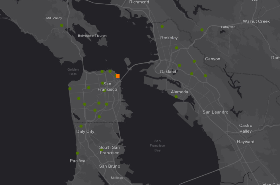
# Call custom function defined earlier in this notebook to
# display the analysis results in the map.
visualize_vehicle_routing_problem_domain(map0, orders_fset=stores_fset,
                                         depots_fset=distribution_center_fset, zoom_level=8)
Once you have all the inputs as featuresets, you can pass inputs converted from different formats. The preparation step shown above is not the only way to do it. For example, depot could be a featureset geocoded from address, orders and routes could be read from csv files to convert to featureset.
Now, we are ready to explore the implementations with three practical examples:
Solution 1: A Basic Scenario
The basic scenario
Assuming that the requirements for the basic scenario is solving the problem of how to dispatch the three trucks in San Francisco (working from 8AM to 5PM) in delivering goods to 25 different stores. In the basic scenario, the distributor is given three required input parameters:
ordersYou will add the grocery store locations to theOrdersfeature class. You can think of orders as orders to be filled, since each grocery store has requested goods to be delivered to it from the distribution center. Members of the Orders class will eventually become stops along the vehicles' routes. The attributes of Stores contain information about the total weight of goods (in pounds) required at each store, the time window during which the delivery has to be made, and the service time (in minutes) incurred while visiting a particular store. The service time is the time required to unload the goods.depotsThe goods are delivered from a single distribution center whose location is shown in theDistributionCenterfeature class. The distribution center operates between 8:00 a.m. and 5:00 p.m.routesThe distribution center has three trucks, each with a maximum capacity to carry 15,000 pounds of goods. You will add three routes (one for each vehicle) and set the properties for the routes based on the center's operational procedures.
Optional Attributes
Other optional attributes include:
- If we need driving directions for navigation, populate_directions must be set to true.
Time Attribute = TravelTime (Minutes)The VRP solver will use this attribute to calculate time-based costs between orders and the depot. Use the default here.Distance Attribute = MetersThis attribute is used to determine travel distances between orders and the depot for constraint purposes and creating directions; however, the VRP solver's objective is to minimize time costs. Use the default here.Default Dateis set to be the day of today (i.e. Monday)Capacity Countis set to 1. This setting indicates that the goods being delivered have only one measurement. In this case, that measurement is weight (pounds). If the capacities were specified in terms of two measurements, such as weight and volume, then the capacity count would be set to 2.- Minutes is selected for
Time Field Units. This specifies that all time-based attributes, such as ServiceTime and MaxViolationTime1 for Orders and MaxTotalTime, MaxTotalTravelTime, and CostPerUnitTime for Route, are in minutes. Distance Field Unitsis set to Miles. This specifies that all distance-based attributes, such as MaxTotalDistance and CostPerUnitDistance for Routes, are in miles.- Since it is difficult for these delivery trucks to make U-turns, set
U-Turns at Junctionsto Not Allowed. - Select between
Straight Line,True Shape with MeasuresorTrue Shape optionfor theOutput Shape Type. Note that this option only affects the display of the routes, not the results determined by the VRP solver. - Using
Use Hierarchyas default here (a.k.a. True).
You can set save_route_data to True if you want to save the route data from result to local disk, which would then be used to upload to online to share with drivers eventually and share the routes in ArcGIS online or Enterprise. Individual routes are saved as route layers which could then be opened in navigator with directions(if you solve with populate_directions=True) (4).
Solve the VRP
The following operations can help you sort out the basic scenario - how to dispatch the three trucks in San Francisco (working from 8AM to 5PM) in delivering goods to 25 different stores. The output will also include the driving directions in Spanish.
Also note that you can set the if_async variable to True, when you need to execute multiple solvers in parallel.
if_async = False%%time
current_date = dt.datetime.now().date()
result1 = network.analysis.solve_vehicle_routing_problem(orders=stores_fset, depots=distribution_center_fset,
default_date=current_date,
routes=routes_fset, populate_route_lines=True,
save_route_data=True,
populate_directions=True,
directions_language="es",
future=if_async)WARNING 030194: Data values longer than 500 characters for field [Routes:StartDepotName] are truncated. WARNING 030194: Data values longer than 500 characters for field [Routes:EndDepotName] are truncated. Network elements with avoid-restrictions are traversed in the output (restriction attribute names: "Through Traffic Prohibited").
Wall time: 17.4 s
The VRP solver calculates the three routes required to service the orders and draws lines connecting the orders. Each route begins and ends at the distribution center and serves a set of orders along the way.
Only when the job is finished and shown as succeeded can we proceed to explore the results. Otherwise, skip the rest of this section and check out the solution 2 instead.
if if_async:
    if result1.done():
        result1 = result1.result()
        print("Async job done!")
    else:
        print("Async job not done yet!")
print('Analysis succeeded? {}'.format(result1.solve_succeeded))
Analysis succeeded? True
Here result1 is a arcgis.geoprocessing._support.ToolOutput Class object, and contains multiple objects - out_routes (FeatureSet), out_stops(FeatureSet), etc. Since that we have enabled save_route_data, out_route_data will appear in the resulting tool output as a dictionary object that is the url pointing to the zipped file of the route data (saved on the GIS object).
result1ToolOutput(out_unassigned_stops=<FeatureSet> 0 features, out_stops=<FeatureSet> 31 features, out_routes=<FeatureSet> 3 features, out_directions=<FeatureSet> 327 features, solve_succeeded=True, out_network_analysis_layer=None, out_route_data={"url": "https://logistics.arcgis.com/arcgis/rest/directories/arcgisjobs/world/vehicleroutingproblem_gpserver/jf37fa7c9adb8401eb25e542a80649b36/scratch/_ags_rd32cf32d6867f46418b1b7b820a24f081.zip"}, out_result_file=None)Tabularizing the response from solve_vehicle_routing_problem
Now, let's explore the tabularized output from solve_vehicle_routing_problem. What will be useful for distributor and the drivers will be the summarized route information, and sequences of stops per route.
# Display the analysis results in a pandas dataframe.
out_routes_df = result1.out_routes.sdf
out_routes_df[['Name','OrderCount','StartTime','EndTime',
'TotalCost','TotalDistance','TotalTime','TotalTravelTime','StartTimeUTC','EndTimeUTC']]| Name | OrderCount | StartTime | EndTime | TotalCost | TotalDistance | TotalTime | TotalTravelTime | StartTimeUTC | EndTimeUTC | |
|---|---|---|---|---|---|---|---|---|---|---|
| 0 | Truck_1 | 8 | 2019-10-16 08:00:00 | 2019-10-16 14:37:08.923000097 | 162.129803 | 55.133374 | 397.148711 | 149.148711 | 2019-10-16 15:00:00 | 2019-10-16 21:37:08.923000097 |
| 1 | Truck_2 | 6 | 2019-10-16 08:00:00 | 2019-10-16 12:22:39.262000084 | 72.355190 | 13.216210 | 262.654374 | 55.654374 | 2019-10-16 15:00:00 | 2019-10-16 19:22:39.262000084 |
| 2 | Truck_3 | 11 | 2019-10-16 08:00:00 | 2019-10-16 15:36:25.043999910 | 186.840470 | 63.704659 | 456.417407 | 145.417407 | 2019-10-16 15:00:00 | 2019-10-16 22:36:25.043999910 |
Based on the dataframe display of the out_routes object, we can tell the optimal routing option provided by solve_vehicle_routing_problem is for Truck_1 to visit 8 stops, Truck_2 to visit 6 stops, and Truck_3 to visit 11 stops. Upon this selection, the total cost will be 162.13 + 72.36 + 186.84 = 421.33, the total distance is 55.13 + 13.22 + 63.70 = 132.05, and the total travel time will be 149.15 + 55.65 + 145.42 = 350.22.
| Scenario | Total Cost | Total Distance | Total Travel Time | Scheduled Stops |
|---|---|---|---|---|
| #1 | 421.33 | 132.05 | 350.22 | [8,6,11] |
out_stops_df = result1.out_stops.sdf
out_stops_df[['Name','RouteName','Sequence','ArriveTime','DepartTime']].sort_values(by=['RouteName',
'Sequence'])| Name | RouteName | Sequence | ArriveTime | DepartTime | |
|---|---|---|---|---|---|
| 25 | San Francisco | Truck_1 | 1 | 2019-10-16 08:00:00.000000000 | 2019-10-16 09:00:00.000000000 |
| 20 | Store_21 | Truck_1 | 2 | 2019-10-16 09:23:24.568000078 | 2019-10-16 09:46:24.568000078 |
| 23 | Store_24 | Truck_1 | 3 | 2019-10-16 09:53:20.523000001 | 2019-10-16 10:17:20.523000001 |
| 19 | Store_20 | Truck_1 | 4 | 2019-10-16 10:35:41.608999968 | 2019-10-16 10:56:41.608999968 |
| 24 | Store_25 | Truck_1 | 5 | 2019-10-16 11:16:34.795000076 | 2019-10-16 11:39:34.795000076 |
| 22 | Store_23 | Truck_1 | 6 | 2019-10-16 11:44:58.622999907 | 2019-10-16 12:02:58.622999907 |
| 9 | Store_10 | Truck_1 | 7 | 2019-10-16 12:15:57.345999956 | 2019-10-16 12:41:57.345999956 |
| 21 | Store_22 | Truck_1 | 8 | 2019-10-16 12:51:14.118000031 | 2019-10-16 13:17:14.118000031 |
| 8 | Store_9 | Truck_1 | 9 | 2019-10-16 13:32:55.437000036 | 2019-10-16 13:59:55.437000036 |
| 26 | San Francisco | Truck_1 | 10 | 2019-10-16 14:37:08.923000097 | 2019-10-16 14:37:08.923000097 |
| 27 | San Francisco | Truck_2 | 1 | 2019-10-16 08:00:00.000000000 | 2019-10-16 09:00:00.000000000 |
| 18 | Store_19 | Truck_2 | 2 | 2019-10-16 09:01:38.371999979 | 2019-10-16 09:29:38.371999979 |
| 17 | Store_18 | Truck_2 | 3 | 2019-10-16 09:35:04.229000092 | 2019-10-16 09:53:04.229000092 |
| 16 | Store_17 | Truck_2 | 4 | 2019-10-16 09:57:35.167000055 | 2019-10-16 10:24:35.167000055 |
| 14 | Store_15 | Truck_2 | 5 | 2019-10-16 10:33:28.065999985 | 2019-10-16 10:54:28.065999985 |
| 2 | Store_3 | Truck_2 | 6 | 2019-10-16 11:02:16.391999960 | 2019-10-16 11:26:16.391999960 |
| 15 | Store_16 | Truck_2 | 7 | 2019-10-16 11:37:30.953000069 | 2019-10-16 12:06:30.953000069 |
| 28 | San Francisco | Truck_2 | 8 | 2019-10-16 12:22:39.262000084 | 2019-10-16 12:22:39.262000084 |
| 29 | San Francisco | Truck_3 | 1 | 2019-10-16 08:00:00.000000000 | 2019-10-16 09:00:00.000000000 |
| 7 | Store_8 | Truck_3 | 2 | 2019-10-16 09:28:19.667000055 | 2019-10-16 09:54:19.667000055 |
| 0 | Store_1 | Truck_3 | 3 | 2019-10-16 10:17:51.694000006 | 2019-10-16 10:42:51.694000006 |
| 1 | Store_2 | Truck_3 | 4 | 2019-10-16 10:50:28.684999943 | 2019-10-16 11:13:28.684999943 |
| 3 | Store_4 | Truck_3 | 5 | 2019-10-16 11:19:50.032000065 | 2019-10-16 11:39:50.032000065 |
| 6 | Store_7 | Truck_3 | 6 | 2019-10-16 11:49:47.717000008 | 2019-10-16 12:06:47.717000008 |
| 5 | Store_6 | Truck_3 | 7 | 2019-10-16 12:14:38.335999966 | 2019-10-16 12:40:38.335999966 |
| 10 | Store_11 | Truck_3 | 8 | 2019-10-16 12:50:19.503999949 | 2019-10-16 13:08:19.503999949 |
| 11 | Store_12 | Truck_3 | 9 | 2019-10-16 13:21:35.124000072 | 2019-10-16 13:43:35.124000072 |
| 4 | Store_5 | Truck_3 | 10 | 2019-10-16 13:49:50.144000053 | 2019-10-16 14:10:50.144000053 |
| 12 | Store_13 | Truck_3 | 11 | 2019-10-16 14:17:07.040999889 | 2019-10-16 14:44:07.040999889 |
| 13 | Store_14 | Truck_3 | 12 | 2019-10-16 14:49:39.961999893 | 2019-10-16 15:15:39.961999893 |
| 30 | San Francisco | Truck_3 | 13 | 2019-10-16 15:36:25.043999910 | 2019-10-16 15:36:25.043999910 |
Visualizing the response from from solve_vehicle_routing_problem
In order to improve the re-usability of codes, we will define a method called visualize_vehicle_routing_problem_results to render the map, and visualize the orders, depots and the routing results calculated by the VRP solver. This method will be reused in scenarios 2 and 3 as well.
# Define the route symbols as blue, red and green
route_symbols = [SimpleLineSymbolEsriSLS(**{"type": "esriSLS",
                          "style": "esriSLSSolid",
                          "color": [0,100,240,255],"size":10}),
                 SimpleLineSymbolEsriSLS(**{"type": "esriSLS",
                          "style": "esriSLSSolid",
                          "color": [255,0,0,255],"size":10}),
                 SimpleLineSymbolEsriSLS(**{"type": "esriSLS",
                          "style": "esriSLSSolid",
                          "color": [100,240,0,255],"size":10})]

# Define a function to display the output analysis results in a map
def visualize_vehicle_routing_problem_results(map_widget, solve_vehicle_routing_problem_result,
                                              orders_fset, depots_fset, zoom_level,
                                              route_zones_fset = None):
    # The map widget
    map_view_outputs = map_widget
    # The solve_vehicle_routing_problem analysis result
    results = solve_vehicle_routing_problem_result

    #Visusalize the inputs with different symbols
    map_view_outputs.content.draw(orders_fset, symbol=SimpleMarkerSymbolEsriSMS(**{"type": "esriSMS",
                                               "style": "esriSMSCircle",
                                               "color": [76,115,0,255],"size": 8}))
    map_view_outputs.content.draw(depots_fset, symbol=SimpleMarkerSymbolEsriSMS(**{"type": "esriSMS",
                                               "style": "esriSMSSquare",
                                               "color": [255,115,0,255], "size": 10}))
    if route_zones_fset is not None:
        route_zones_sym = SimpleFillSymbolEsriSFS(**{
            "type": "esriSFS",
            "style": "esriSFSSolid",
            "color": [255,165,0,0],
            "outline": {
                "type": "esriSLS",
                "style": "esriSLSSolid",
                "color": [255,0,0,255],
                "width": 4}
        })
        map_view_outputs.content.draw(route_zones_fset, symbol=route_zones_sym)

    #Visualize each route
    for i in range(len(results.out_routes.features)):
        out_routes_flist = []
        out_routes_flist.append(results.out_routes.features[i])
        out_routes_fset = []
        out_routes_fset = FeatureSet(out_routes_flist)
        map_view_outputs.draw(out_routes_fset,
                              symbol=route_symbols[i%3])

    # Zoom out to display all of the allocated census points.
    map_view_outputs.zoom = zoom_level
# Display the analysis results in a map.
# Create a map of SF, California.
map1 = my_gis.map('San Francisco, CA')
map1.basemap.basemap = 'dark-gray-vector'
map1
# Call custom function defined earlier in this notebook to
# display the analysis results in the map.
visualize_vehicle_routing_problem_results(map1, result1,
                                          orders_fset=stores_fset, depots_fset=distribution_center_fset, zoom_level=8)
Judging from what's displayed in map1, Truck_1 (blue) tends to take care of the stores located at the east side of San Francisco, while the Truck_2 (red) and Truck_3 (green) are responsible for delivering goods to stores located at the west. Also, the difference between Truck_2 and Truck_3 is that the former handles the downtown area, and the latter focuses on the outer rim.
Animating the response from from solve_vehicle_routing_problem
In order to show a stronger sequential relationship between origin, stops and destination of each solved route, we can also use animate_vehicle_routing_problem_results function to be defined below, to animate each stop along the route sequentially:
# Display the analysis results in a map.

# Create a map of SF, California.
map1a = my_gis.map('San Francisco, CA')
map1a.basemap.basemap = 'dark-gray-vector'
map1a
"""Used to convert 1 to A, 2 to B, and 3 to C, in order to compose the symbol url
"""
def int_to_letter(num):
    alphabet = list('ABCDEFGHIJKLMNOPQRSTUVWXYZ')
    return alphabet[num-1]


"""Used to construct the symbol url, in which route color and sequence is annotated
"""
def create_stops_symbol_url(sequence_number, route_name):
    base_url = "http://static.arcgis.com/images/Symbols/AtoZ/"
    if route_name == 'Truck_1': #Blue
        color = 'blue'
    elif route_name == 'Truck_2': #Red
        color = 'red'
    else: #Green
        color = 'green'
    return base_url + color + int_to_letter(sequence_number) + ".png"


"""Used to create the symbol dict aiming for map rendering
"""
def get_stops_symbol(sequence_number, route_name):
    stops_symbol = PictureMarkerSymbolEsriPMS(**{"angle":0,"xoffset":0,"yoffset":8.15625,"type":"esriPMS",
                    "url":create_stops_symbol_url(sequence_number, route_name),
                    "contentType":"image/png","width":15.75,"height":21.75})
    return stops_symbol


"""When the sequence number is 1 or the max, join stops_df with depot_fset, and draw on map
"""
def draw_origin_destination(number, route_name, map_widget, out_stops_df, reference_sdf = None):

    df = out_stops_df[out_stops_df['Sequence'] == number]
    if df is not None and len(df) > 0:
        df = df[df['RouteName'] == route_name][['ObjectID', 'Sequence', 'Name', 'RouteName']]
        if df is not None and len(df) > 0:
            if reference_sdf is None:
                reference_sdf = distribution_center_fset.sdf[['OBJECTID', 'SHAPE', 'NAME']]
                reference_sdf['Name'] = reference_sdf['NAME']
                del reference_sdf['NAME']

            df3 = pd.merge(df, reference_sdf, on='Name', how='inner')
            df3.spatial.plot(map_widget, symbol=get_stops_symbol(number, route_name))
            print(number)


"""When the sequence number is between 1 and max, join stops_df with orders_fset, and draw on map
"""
def draw_stops(number, route_name, map_widget, out_stops_df, reference_sdf = None):

    df = out_stops_df[out_stops_df['Sequence'] == number]
    if df is not None and len(df) > 0:
        df = df[df['RouteName'] == route_name][['ObjectID', 'Sequence', 'Name', 'RouteName']]
        if df is not None and len(df) > 0:
            if reference_sdf is None:
                reference_sdf = stores_fset.sdf[['OBJECTID', 'SHAPE', 'NAME']]
                reference_sdf['Name'] = reference_sdf['NAME']
                del reference_sdf['NAME']

            df3 = pd.merge(df, reference_sdf, on='Name', how='inner')
            if df3 is not None and len(df3) > 0:
                df3.spatial.plot(map_widget, symbol=get_stops_symbol(number, route_name))
            print(number)


"""Assign 0 to Truck_1, 1 to Truck_2, and 2 to Truck_3
"""
def get_route_color_index(route_name):
    return int(route_name[-1])-1


"""Visualize the origin, stops, and destination along each set of routing options,
   based on various color for route[0], [1] and [2], with a time sleep of 1 sec per stop
"""
# Define a function to display the output analysis results in a map
def animate_vehicle_routing_problem_results(map_widget, solve_vehicle_routing_problem_result,
                                            orders_fset, depots_fset, zoom_level = None,
                                            route_zones_fset = None):
    # The map widget
    map_view_outputs = map_widget
    # The solve_vehicle_routing_problem analysis result
    results = solve_vehicle_routing_problem_result

    map_view_outputs.content.remove_all()

    #Visusalize the inputs with different symbols
    map_view_outputs.content.draw(orders_fset, symbol=SimpleMarkerSymbolEsriSMS(**{"type": "esriSMS",
                                               "style": "esriSMSCircle",
                                               "color": [76,115,0,255],"size": 8}))
    map_view_outputs.content.draw(depots_fset, symbol=SimpleMarkerSymbolEsriSMS(**{"type": "esriSMS",
                                               "style": "esriSMSSquare",
                                               "color": [255,115,0,255], "size": 10}))
    if route_zones_fset is not None:
        route_zones_sym = SimpleFillSymbolEsriSFS(**{
            "type": "esriSFS",
            "style": "esriSFSSolid",
            "color": [255,165,0,0],
            "outline": {
                "type": "esriSLS",
                "style": "esriSLSSolid",
                "color": [255,0,0,255],
                "width": 4}
        })
        map_view_outputs.content.draw(route_zones_fset, symbol=route_zones_sym)

    #Visualize each route
    for i in range(len(results.out_routes.features)):
        out_routes_flist = []
        out_routes_flist.append(results.out_routes.features[i])
        out_routes_fset = []
        out_routes_fset = FeatureSet(out_routes_flist)

        route_name = results.out_routes.features[i].attributes['Name']
        color_index = get_route_color_index(route_name)

        map_view_outputs.content.draw(out_routes_fset,
                              symbol=route_symbols[color_index])

    #Visualize each stop
    reference_sdf0 = distribution_center_fset.sdf[['OBJECTID', 'SHAPE', 'NAME']]
    reference_sdf0['Name'] = reference_sdf0['NAME']
    del reference_sdf0['NAME']

    reference_sdf = stores_fset.sdf[['OBJECTID', 'SHAPE', 'NAME']]
    reference_sdf['Name'] = reference_sdf['NAME']
    del reference_sdf['NAME']

    out_stops_df = results.out_stops.sdf
    time.sleep(5)
    for route in ['Truck_1', 'Truck_2', 'Truck_3']:
        df = out_stops_df[out_stops_df['RouteName'] == route]
        max_stops_cnt = len(df)
        for i in range(max_stops_cnt):
            if i>0 and i<max_stops_cnt-1:
                draw_stops(i+1, route, map_view_outputs, df, reference_sdf)
            else:
                draw_origin_destination(i+1, route, map_view_outputs, df, reference_sdf0)
            time.sleep(1)

    # Zoom out to display all of the allocated census points.
    if zoom_level is not None:
        map_view_outputs.zoom = zoom_level
# Call custom function defined earlier in this notebook to
# animate the analysis results in the map.
animate_vehicle_routing_problem_results(map1a, result1,
orders_fset=stores_fset, depots_fset=distribution_center_fset)Saving the response from from solve_vehicle_routing_problem to online
Save the route data from result to local disk, which would then be used to upload to online portal to share with drivers eventually and share the routes in ArcGIS online on the portal. Individual routes are saved as route layers which could then be opened in navigator with directions(if you solve with 'populate_directions'=true')
route_data = result1.out_route_data.download('.')
root_folder = my_gis.content.folders.get()
route_data_item = root_folder.add({"type": "File Geodatabase"}, route_data).result()
route_data_item
Then, to create route layers from the route data. This will create route layers in the online or enterprise which could then be shared with drivers, so they would be able to open this in navigator.
route_layers = analysis.create_route_layers(route_data_item,
                                            delete_route_data_item=True)
for route_layer in route_layers:
    route_layer.share(org=True)
    display(route_layer.homepage)
    display(route_layer)
'https://your_target_gis/home/item.html?id=6d41dbd910124ec88e941b98d8175220'
'https://your_target_gis/home/item.html?id=c71c297e83904a9fac183f9c4864bfed'
'https://your_target_gis/home/item.html?id=02a63587c34048d9bfd9377c39ad7ae7'
A second solver in arcgis.features module
Now let's look at a second solver in arcgis.features module that can also solve a vehicle routing problem, with a Feature service (input) to (Feature Service) approach. Parameters for this solver include:
route_count: Required integer. The number of vehicles that are available to visit the stops. The method supports up to 100 vehicles. The default value is 0.max_stops_per_route: Required integer. The maximum number of stops a route, or vehicle, is allowed to visit. The largest value you can specify is 200. The default value is zero.start_layer: Required feature layer. Provide the locations where the people or vehicles start their routes. You can specify one or many starting locations. In this case, the distribution center.return_to_start: default is True. When set to False, user has to provide theend_layer.stop_service_time: Optional float. Indicates how much time, in minutes, is spent at each stop. The units are minutes. All stops are assigned the same service duration from this parameter — unique values for individual stops cannot be specified with this service.include_route_layers: Optional boolean. When include_route_layers is set to True, each route from the result is also saved as a route layer item.output_name: Optional string. If provided, the method will create a feature service of the results. You define the name of the service. If output_name is not supplied, the method will return a feature collection.
from arcgis.features.analysis import plan_routes

result1b = plan_routes(stops_layer=stores_fl,
                       route_count=3,
                       max_stops_per_route=15,
                       route_start_time=dt.datetime(2019, 10, 16, 8, 0),
                       start_layer=distribution_center_fl,
                       return_to_start=True,
                       travel_mode='Driving Time',
                       stop_service_time=23.44,
                       include_route_layers=False,
                       output_name='plan route for grocery stores')
Network elements with avoid-restrictions are traversed in the output (restriction attribute names: "Through Traffic Prohibited").
result1bvrp_sublayer = FeatureLayer.fromitem(result1b, layer_id=0)
vrp_df = vrp_sublayer.query(where='1=1', as_df=True)
# filter only the required columns
vrp_df2 = vrp_df[['OBJECTID', 'NAME','RouteName', 'StopType','ArriveTime','DepartTime','Demand','FromPrevDistance','FromPrevTravelTime']]
vrp_df2| OBJECTID | NAME | RouteName | StopType | ArriveTime | DepartTime | Demand | FromPrevDistance | FromPrevTravelTime | |
|---|---|---|---|---|---|---|---|---|---|
| 0 | 1 | None | San Francisco - Route1 | Route start | 2019-10-16 15:00:00 | 2019-10-16 15:00:00 | NaN | 0.000000 | 0.000000 |
| 1 | 2 | Store_9 | San Francisco - Route1 | Stop | 2019-10-16 15:30:17 | 2019-10-16 15:53:43 | 1815.0 | 13.069925 | 30.277377 |
| 2 | 3 | Store_22 | San Francisco - Route1 | Stop | 2019-10-16 16:09:32 | 2019-10-16 16:32:58 | 1767.0 | 4.681508 | 15.808563 |
| 3 | 4 | Store_10 | San Francisco - Route1 | Stop | 2019-10-16 16:46:39 | 2019-10-16 17:10:05 | 1709.0 | 6.056615 | 13.678811 |
| 4 | 5 | Store_23 | San Francisco - Route1 | Stop | 2019-10-16 17:19:54 | 2019-10-16 17:43:20 | 1053.0 | 6.257358 | 9.812247 |
| 5 | 6 | Store_25 | San Francisco - Route1 | Stop | 2019-10-16 17:47:24 | 2019-10-16 18:10:51 | 1469.0 | 2.508181 | 4.065832 |
| 6 | 7 | Store_24 | San Francisco - Route1 | Stop | 2019-10-16 18:17:37 | 2019-10-16 18:41:03 | 1593.0 | 2.366756 | 6.768300 |
| 7 | 8 | Store_21 | San Francisco - Route1 | Stop | 2019-10-16 18:47:00 | 2019-10-16 19:10:26 | 1525.0 | 2.828495 | 5.942969 |
| 8 | 9 | Store_20 | San Francisco - Route1 | Stop | 2019-10-16 19:29:49 | 2019-10-16 19:53:15 | 1364.0 | 8.690247 | 19.379384 |
| 9 | 10 | None | San Francisco - Route1 | Route end | 2019-10-16 20:31:24 | 2019-10-16 20:31:24 | NaN | 14.764634 | 38.150011 |
| 10 | 11 | None | San Francisco - Route2 | Route start | 2019-10-16 15:00:00 | 2019-10-16 15:00:00 | NaN | 0.000000 | 0.000000 |
| 11 | 12 | Store_19 | San Francisco - Route2 | Stop | 2019-10-16 15:01:38 | 2019-10-16 15:25:05 | 1950.0 | 0.295987 | 1.639528 |
| 12 | 13 | Store_18 | San Francisco - Route2 | Stop | 2019-10-16 15:30:31 | 2019-10-16 15:53:57 | 1056.0 | 1.310270 | 5.430962 |
| 13 | 14 | Store_17 | San Francisco - Route2 | Stop | 2019-10-16 15:58:28 | 2019-10-16 16:21:54 | 1872.0 | 1.187248 | 4.515628 |
| 14 | 15 | Store_15 | San Francisco - Route2 | Stop | 2019-10-16 16:30:47 | 2019-10-16 16:54:14 | 1373.0 | 1.721283 | 8.881646 |
| 15 | 16 | Store_16 | San Francisco - Route2 | Stop | 2019-10-16 17:01:09 | 2019-10-16 17:24:35 | 1962.0 | 1.222963 | 6.920458 |
| 16 | 17 | None | San Francisco - Route2 | Route end | 2019-10-16 17:40:44 | 2019-10-16 17:40:44 | NaN | 3.464067 | 16.138486 |
| 17 | 18 | None | San Francisco - Route3 | Route start | 2019-10-16 15:00:00 | 2019-10-16 15:00:00 | NaN | 0.000000 | 0.000000 |
| 18 | 19 | Store_8 | San Francisco - Route3 | Stop | 2019-10-16 15:28:20 | 2019-10-16 15:51:46 | 1761.0 | 12.772203 | 28.327778 |
| 19 | 20 | Store_3 | San Francisco - Route3 | Stop | 2019-10-16 16:11:43 | 2019-10-16 16:35:09 | 1580.0 | 10.551517 | 19.942193 |
| 20 | 21 | Store_1 | San Francisco - Route3 | Stop | 2019-10-16 16:42:12 | 2019-10-16 17:05:38 | 1706.0 | 2.625955 | 7.042673 |
| 21 | 22 | Store_2 | San Francisco - Route3 | Stop | 2019-10-16 17:13:15 | 2019-10-16 17:36:41 | 1533.0 | 2.465322 | 7.616514 |
| 22 | 23 | Store_4 | San Francisco - Route3 | Stop | 2019-10-16 17:43:03 | 2019-10-16 18:06:29 | 1289.0 | 1.547229 | 6.355779 |
| 23 | 24 | Store_13 | San Francisco - Route3 | Stop | 2019-10-16 18:13:44 | 2019-10-16 18:37:10 | 1863.0 | 2.158465 | 7.244590 |
| 24 | 25 | Store_14 | San Francisco - Route3 | Stop | 2019-10-16 18:42:43 | 2019-10-16 19:06:09 | 1791.0 | 1.386497 | 5.548683 |
| 25 | 26 | Store_5 | San Francisco - Route3 | Stop | 2019-10-16 19:11:59 | 2019-10-16 19:35:26 | 1302.0 | 2.069020 | 5.832916 |
| 26 | 27 | Store_12 | San Francisco - Route3 | Stop | 2019-10-16 19:41:58 | 2019-10-16 20:05:24 | 1414.0 | 1.751279 | 6.527311 |
| 27 | 28 | Store_7 | San Francisco - Route3 | Stop | 2019-10-16 20:13:37 | 2019-10-16 20:37:03 | 1014.0 | 3.428752 | 8.214252 |
| 28 | 29 | Store_6 | San Francisco - Route3 | Stop | 2019-10-16 20:44:54 | 2019-10-16 21:08:20 | 1775.0 | 4.629602 | 7.843654 |
| 29 | 30 | Store_11 | San Francisco - Route3 | Stop | 2019-10-16 21:18:01 | 2019-10-16 21:41:28 | 1045.0 | 6.470590 | 9.686140 |
| 30 | 31 | None | San Francisco - Route3 | Route end | 2019-10-16 22:08:35 | 2019-10-16 22:08:35 | NaN | 12.806232 | 27.119240 |
vrp_sublayer_b = FeatureLayer.fromitem(result1b, layer_id=1)
vrp_df_b = vrp_sublayer_b.query(where='1=1', as_df=True)

# filter only the required columns
vrp_df2_b = vrp_df_b[['OBJECTID', 'RouteName', 'StartTime','EndTime','StopCount','TotalTime','TotalTravelTime','Total_Miles']]
vrp_df2_b| OBJECTID | RouteName | StartTime | EndTime | StopCount | TotalTime | TotalTravelTime | Total_Miles | |
|---|---|---|---|---|---|---|---|---|
| 0 | 1 | San Francisco - Route1 | 2019-10-16 15:00:00 | 2019-10-16 20:31:24 | 8 | 331.403494 | 143.883494 | 61.223720 |
| 1 | 2 | San Francisco - Route2 | 2019-10-16 15:00:00 | 2019-10-16 17:40:44 | 5 | 160.726708 | 43.526708 | 9.201818 |
| 2 | 3 | San Francisco - Route3 | 2019-10-16 15:00:00 | 2019-10-16 22:08:35 | 12 | 428.581722 | 147.301722 | 64.662664 |
Compared to the result we have got from network.analysis solver, the schedules provided by plan_routes are slightly different:
| Scenario | Total Cost | Total Distance | Total Travel Time | Scheduled Stops |
|---|---|---|---|---|
| #1 | 421.33 | 132.05 | 350.22 | [8,6,11] |
| #1b | 421.33 | 135.09 | 334.712 | [8,5,12] |
Different algorithms underneath these two solvers can be one of the reasons that lead to the variance. Also, the service time for each stop in the stops layer is different, from 17 to 29 minutes, and this attribute is taken into consideration by the network.analysis.solve_vehicle_routing_problem tool. However, the arcgis.features.analysis.plan_routes is limited from this perspective since all stops are assigned the same service duration (in this case 23.44 minutes, the average of service time for all stops) from this parameter — unique values for individual stops cannot be specified with this service.
# Display the analysis results in a map.

# Create a map of SF, California.
map1b = my_gis.map('San Francisco, CA')
map1b.basemap.basemap = 'dark-gray-vector'
map1b
The layer (id=0) contains stops scheduled to be visited by Truck_1, Truck_2 and Truck_3 respectively.
The layer (id=1) lists three planned routes for Truck_1, Truck_2 and Truck_3
for i in range(2):
    map1b.content.add(FeatureLayer(result1b.url + "/" + str(i)))
In the last section, we have adopted a different method - arcgis.features.use_proximity.plan_routes - in solving a VRP. In doing so, we also explored the scenario with output_name specified (which forms a Feature Service to Feature Service user experience). Note that, though plan_routes is workflow-driven and provides more user-friendly input/output interface, there are limitations to its implementation. As seen in the example above, the service time is set as a constant float while solve_vehicle_routing_problem can consider this attribute as variables.
Next, we will explore more complicated scenarios with the solve_vehicle_routing_problem tool.
Solution 2: A modified scenario
The vehicle routing problem solution obtained earlier worked well for the company. After a few weeks, however, the driver assigned to Truck_2 went on vacation. So now the distribution company has to service the same stores but with just two trucks. To accommodate the extra workload, the company decided to pay overtime to the other two drivers and provide them with one paid break during the day. The distribution company also acquired two additional satellite distribution centers. These centers can be used by the trucks to renew their truckload while making their deliveries instead of returning to the main distribution center for renewal. You will modify the solution obtained from the previous solution to accommodate these changes.
- delete an existing route, and modify
routesto include overtime - add
route renewals - modify the
depotsfeature class - add
breaks - again, determine the solution
Solve the VRP
Step 1: Modify the routes feature class
When MaxTotalTime is set to 540, that means drivers can't have a work shift of more than nine hours (a.k.a. from 8AM to 5PM). When MaxTotalTime is "Null", that means drivers are allowed to work on overtime shift.
Here, we have specified MaxTotalTime to be 600 which means drivers are not allowed to work more than 10 hours (including the break times), and the OverTimeStartTime is set to 480 meaning that all hours over 8 would be charged overtime.
route_csv2 = "data/vrp/routes_solution2.csv"

# Read the csv file
route_df2 = pd.read_csv(route_csv2)
route_df2| ObjectID | Name | StartDepotName | EndDepotName | StartDepotServiceTime | EarliestStartTime | LatestStartTime | Capacities | CostPerUnitTime | CostPerUnitDistance | MaxTotalTime | MaxTotalTravelTime | MaxTotalDistance | AssignmentRule | OvertimeStartTime | CostPerUnitOvertime | MaxOrderCount | |
|---|---|---|---|---|---|---|---|---|---|---|---|---|---|---|---|---|---|
| 0 | 1 | Truck_1 | San Francisco | San Francisco | 60 | 8:00:00 | 8:00:00 | 15000 | 0.2 | 1.5 | 600 | <Null> | <Null> | 1 | 480 | 0.3 | 20 |
| 1 | 2 | Truck_3 | San Francisco | San Francisco | 60 | 8:00:00 | 8:00:00 | 15000 | 0.2 | 1.5 | 600 | <Null> | <Null> | 1 | 480 | 0.3 | 20 |
routes_fset2 = FeatureSet.from_dataframe(route_df2)
display(routes_fset2)
<FeatureSet> 2 features
Step 2: add a new route_renewals feature class
In some cases, a depot can also act as a renewal location whereby the vehicle can unload or reload and continue performing deliveries and pickups. A depot has open and close times, as specified by a hard time window. Vehicles can’t arrive at a depot outside of this time window.
The StartDepotName and EndDepotName fields of the Routes record set reference the names you specify here. It is also referenced by the Route Renewals record set, when used.
If the StartDepotName value is null, the route will begin from the first order assigned. Omitting the start depot is useful when the vehicle’s starting location is unknown or irrelevant to your problem. However, when StartDepotName is null, EndDepotName cannot also be null.
If the route is making deliveries and StartDepotName is null, it is assumed the cargo is loaded on the vehicle at a virtual depot before the route begins. For a route that has no renewal visits, its delivery orders (those with nonzero DeliveryQuantities values in the Orders class) are loaded at the start depot or virtual depot. For a route that has renewal visits, only the delivery orders before the first renewal visit are loaded at the start depot or virtual depot.
route_renewals: Route Renewals (FeatureSet). Optional parameter. Specifies the intermediate depots that routes can visit to
reload or unload the cargo they are delivering or picking up. Specifically, a route renewal links a route to a depot. The relationship indicates the route can renew (reload or unload while en route) at the associated depot.
Route renewalscan be used to model scenarios in which a vehicle picks up a full load of deliveries at the starting depot, services the orders, returns to the depot to renew its load of deliveries, and continues servicing more orders. For example, in propane gas delivery, the vehicle may make several deliveries until its tank is nearly or completely depleted, visit a refueling point, and make more deliveries.- Here are a few rules and options to consider when also working with route seed points:
- The reload/unload point, or renewal location, can be different from the start or end depot.
- Each route can have one or many predetermined renewal locations.
- A renewal location may be used more than once by a single route.
- In some cases where there may be several potential renewal locations for a route, the closest available renewal location is chosen by the solver.
- When specifying the route renewals, you need to set properties for each one, such as the name of the depot where the route renewal can occur, by using attributes. The route renewals can be specified with the following attributes: ObjectID: The system-managed ID field.
In the following, we will use route_renewals.csv to present the attributes for the two renewal locations for Truck_1 and Truck_3:
route_renewals_csv = "data/vrp/route_renewals.csv"

# Read the csv file
route_renewals_df = pd.read_csv(route_renewals_csv)
route_renewals_df| ObjectID | DepotName | RouteName | ServiceTime | |
|---|---|---|---|---|
| 0 | 1 | 800 Brush St | Truck_1 | 30 |
| 1 | 2 | 100 Old County Rd | Truck_1 | 30 |
| 2 | 3 | 800 Brush St | Truck_3 | 30 |
| 3 | 4 | 100 Old County Rd | Truck_3 | 30 |
route_renewals_fset = FeatureSet.from_dataframe(route_renewals_df)
display(route_renewals_fset)
<FeatureSet> 4 features
Step 3: Update the depots feature class
The two renewal locations are hence acting as depots as well. Let's use the following cell to update the depots feature class, adding the two renewal locations to the original distribution center.
import json
features_list = [{"geometry": {"x": -122.39431795899992, "y": 37.79674801900006, "type": "point",
                               "spatialReference": {"wkid": 4326, "latestWkid": 4326}},
                  "attributes": {"OBJECTID": 1, "NAME": "San Francisco"}},
                 {"geometry": {"x": -122.410679, "y": 37.790419, "type": "point",
                               "spatialReference": {"wkid": 4326, "latestWkid": 4326}},
                  "attributes": {"OBJECTID": 2, "NAME": "800 Brush St"}},
                 {"geometry": {"x": -122.399299, "y": 37.686118, "type": "point",
                               "spatialReference": {"wkid": 4326, "latestWkid": 4326}},
                  "attributes": {"OBJECTID": 3, "NAME": "100 Old County Rd"}}]
json_in_dict = {"features":features_list,
                "objectIdFieldName": "OBJECTID", "globalIdFieldName": "", "spatialReference": {"wkid": 4326, "latestWkid": 4326},
                "geometryType": "esriGeometryPoint", "fields": [{"name": "OBJECTID", "type": "esriFieldTypeOID",
                                                                 "alias": "OBJECTID", "sqlType": "sqlTypeOther"},
                                                                {"name": "NAME", "type": "esriFieldTypeString",
                                                                 "alias": "NAME", "sqlType": "sqlTypeOther",
                                                                 "length": 50}]}
distribution_center_fset2 = FeatureSet.from_json(json.dumps(json_in_dict))
display(distribution_center_fset2)
<FeatureSet> 3 features
Step 4: add a new breaks feature class
Breaks are the rest periods, for the routes in a given vehicle routing problem. A break is associated with exactly one route, and can be taken after completing an order, while en route to an order, or prior to servicing an order. It has a start time and a duration for which the driver may or may not be paid. There are three options for establishing when a break begins: (1) using a time window, (2) a maximum travel time, or (3) a maximum work time (5).
In the CSV file we specified below, the time variable being used is MaxCumulWorkTime, which represents "the maximum amount of work time that can be accumulated before the break is taken. Work time is always accumulated from the beginning of the route." This field is designed to limit how long a person can work until a break is required. In this case, the time unit for the analysis is set to Minutes, MaxCumulWorkTime has a value of 240, and ServiceTime has a value of 30, the driver will get a 30-minute break after 4 hours of work.
Otherwise, you can either use a combination of TimeWindowStart, TimeWindowEnd, and MaxViolationTime, or MaxTravelTimeBetweenBreaks to specify the time attributes. Remember that these options are mutually exclusive, meaning that if e.g. the MaxCumuWorkTime field has a value, then TimeWindowStart, TimeWindowEnd, MaxViolationTime, and MaxTravelTimeBetweenBreaks must be null for an analysis to solve successfully. For more information to these fields, please checkout the REST API Help doc (5).
In the following, the breaks_solution2.csv file contains necessary information to define a breaks feature class, which include objectID, RouteName, ServiceTime, IsPaid, MaxCumulWorkTime, and timeUnits.
breaks_csv = "data/vrp/breaks_solution2.csv"

# Read the csv file
breaks_df = pd.read_csv(breaks_csv)
breaks_df| ObjectID | RouteName | ServiceTime | IsPaid | MaxCumulWorkTime | timeUnits | |
|---|---|---|---|---|---|---|
| 0 | 1 | Truck_1 | 30 | True | 240 | Minutes |
| 1 | 2 | Truck_3 | 30 | True | 240 | Minutes |
breaks_fset = FeatureSet.from_dataframe(breaks_df)
display(breaks_fset)
<FeatureSet> 2 features
Step 5: Run the Solver again
With route_renewals and breaks specified, and the routes modified to only contain two trucks, the VRP solver now calculates the two routes that can be used to service the orders and draws lines connecting the orders. Each route begins and ends at the distribution center, serves a set of orders along the way, visits a renewal location to load the truck again, continues to service the remaining orders, and finally returns to the distribution center.
if_async = Falseresult2 = network.analysis.solve_vehicle_routing_problem(orders=stores_fset, depots=distribution_center_fset2,
routes=routes_fset2,
route_renewals=route_renewals_fset,
breaks=breaks_fset,
default_date=current_date,
impedance="TruckTravelTime",
time_impedance="TruckTravelTime",
populate_route_lines=True,
populate_directions=True,
directions_language="es",
future=if_async)WARNING 030194: Data values longer than 500 characters for field [Routes:StartDepotName] are truncated. WARNING 030194: Data values longer than 500 characters for field [Routes:EndDepotName] are truncated. WARNING 030194: Data values longer than 500 characters for field [RouteRenewals:DepotName] are truncated. Network elements with avoid-restrictions are traversed in the output (restriction attribute names: "Through Traffic Prohibited").
if if_async:
    if result2.done():
        result2 = result2.result()
        print("Async job done!")
    else:
        print("Async job not done yet!")
print('Analysis succeeded? {}'.format(result2.solve_succeeded))
Analysis succeeded? True
Here result2 is a arcgis.geoprocessing._support.ToolOutput Class object, and contains multiple objects - out_routes (FeatureSet), out_stops(FeatureSet), etc. Since that we have not specified save_route_data, out_route_data will appear in the resulting tooloutput as None.
result2ToolOutput(out_unassigned_stops=<FeatureSet> 0 features, out_stops=<FeatureSet> 31 features, out_routes=<FeatureSet> 2 features, out_directions=<FeatureSet> 313 features, solve_succeeded=True, out_network_analysis_layer=None, out_route_data=None, out_result_file=None)
# Display the analysis results in a pandas dataframe.
out_routes_df = result2.out_routes.sdf
out_routes_df[['Name','OrderCount','StartTime','EndTime',
'TotalCost','TotalDistance','TotalTime','TotalTravelTime']]| Name | OrderCount | StartTime | EndTime | TotalCost | TotalDistance | TotalTime | TotalTravelTime | |
|---|---|---|---|---|---|---|---|---|
| 0 | Truck_1 | 9 | 2019-10-16 08:00:00 | 2019-10-16 16:00:17.405999899 | 207.453092 | 74.244041 | 480.290101 | 176.290101 |
| 1 | Truck_3 | 16 | 2019-10-16 08:00:00 | 2019-10-16 17:56:16.168999910 | 200.988840 | 46.738665 | 596.269478 | 134.269478 |
Note here, the table above is obtained when the time attribute of breaks feature class is set to be using MaxCumulWorkTime. The optimal routing solution is for truck_1 to visit 9 stops and truck_3 to visit 16, and hence the total cost is 207.45 + 200.99 = 408.44 with a total distance of 74.24 + 46.74 = 120.98, and a total travel time of 176.29 + 134.27 = 310.56.
However, alternatively, if we used a combination of TimeWindowStart, TimeWindowEnd, and MaxViolationTime, e.g. trucks have to be operated from 8AM to 5PM, then we can see, the optimal routing option is that truck_1 visited 11 stops while truck_3 visited 14, and the total cost is 236.65 + 194.68 = 431.33 with a total distance of 74.46 + 46.19 = 120.65.
Comparing to the results we have got from solution 1, we can look at this table:
| Scenario | Total Cost | Total Distance | Total Travel Time | Scheduled Stops |
|---|---|---|---|---|
| #1 | 421.33 | 132.05 | 350.22 | [8,6,11] |
| #2 | 408.44 | 120.98 | 310.56 | [9,0,16] |
out_stops_df = result2.out_stops.sdf
out_stops_df[['Name','RouteName','Sequence','ArriveTime','DepartTime']].sort_values(by=['RouteName',
'Sequence'])| Name | RouteName | Sequence | ArriveTime | DepartTime | |
|---|---|---|---|---|---|
| 25 | San Francisco | Truck_1 | 1 | 2019-10-16 08:00:00.000000000 | 2019-10-16 09:00:00.000000000 |
| 20 | Store_21 | Truck_1 | 2 | 2019-10-16 09:23:24.568000078 | 2019-10-16 09:46:24.568000078 |
| 23 | Store_24 | Truck_1 | 3 | 2019-10-16 09:53:20.523000001 | 2019-10-16 10:17:20.523000001 |
| 19 | Store_20 | Truck_1 | 4 | 2019-10-16 10:35:41.608999968 | 2019-10-16 10:56:41.608999968 |
| 24 | Store_25 | Truck_1 | 5 | 2019-10-16 11:16:34.795000076 | 2019-10-16 11:39:34.795000076 |
| 29 | Break | Truck_1 | 6 | 2019-10-16 11:45:00.510999918 | 2019-10-16 12:15:00.510999918 |
| 22 | Store_23 | Truck_1 | 7 | 2019-10-16 12:15:00.510999918 | 2019-10-16 12:33:00.510999918 |
| 9 | Store_10 | Truck_1 | 8 | 2019-10-16 12:45:59.936000109 | 2019-10-16 13:11:59.936000109 |
| 21 | Store_22 | Truck_1 | 9 | 2019-10-16 13:21:21.052999973 | 2019-10-16 13:47:21.052999973 |
| 8 | Store_9 | Truck_1 | 10 | 2019-10-16 14:03:02.371999979 | 2019-10-16 14:30:02.371999979 |
| 7 | Store_8 | Truck_1 | 11 | 2019-10-16 15:02:48.959000111 | 2019-10-16 15:28:48.959000111 |
| 26 | San Francisco | Truck_1 | 12 | 2019-10-16 16:00:17.405999899 | 2019-10-16 16:00:17.405999899 |
| 27 | San Francisco | Truck_3 | 1 | 2019-10-16 08:00:00.000000000 | 2019-10-16 09:00:00.000000000 |
| 18 | Store_19 | Truck_3 | 2 | 2019-10-16 09:01:38.371999979 | 2019-10-16 09:29:38.371999979 |
| 17 | Store_18 | Truck_3 | 3 | 2019-10-16 09:35:04.229000092 | 2019-10-16 09:53:04.229000092 |
| 16 | Store_17 | Truck_3 | 4 | 2019-10-16 09:57:35.167000055 | 2019-10-16 10:24:35.167000055 |
| 14 | Store_15 | Truck_3 | 5 | 2019-10-16 10:33:28.065999985 | 2019-10-16 10:54:28.065999985 |
| 2 | Store_3 | Truck_3 | 6 | 2019-10-16 11:02:16.391999960 | 2019-10-16 11:26:16.391999960 |
| 0 | Store_1 | Truck_3 | 7 | 2019-10-16 11:33:18.951999903 | 2019-10-16 11:58:18.951999903 |
| 30 | Break | Truck_3 | 8 | 2019-10-16 12:00:00.000000000 | 2019-10-16 12:30:00.000000000 |
| 1 | Store_2 | Truck_3 | 9 | 2019-10-16 12:35:55.943000078 | 2019-10-16 12:58:55.943000078 |
| 3 | Store_4 | Truck_3 | 10 | 2019-10-16 13:05:17.289999962 | 2019-10-16 13:25:17.289999962 |
| 6 | Store_7 | Truck_3 | 11 | 2019-10-16 13:35:14.974999905 | 2019-10-16 13:52:14.974999905 |
| 5 | Store_6 | Truck_3 | 12 | 2019-10-16 14:00:05.858999968 | 2019-10-16 14:26:05.858999968 |
| 10 | Store_11 | Truck_3 | 13 | 2019-10-16 14:35:55.555999994 | 2019-10-16 14:53:55.555999994 |
| 11 | Store_12 | Truck_3 | 14 | 2019-10-16 15:07:42.703999996 | 2019-10-16 15:29:42.703999996 |
| 4 | Store_5 | Truck_3 | 15 | 2019-10-16 15:35:57.723999977 | 2019-10-16 15:56:57.723999977 |
| 12 | Store_13 | Truck_3 | 16 | 2019-10-16 16:03:14.621999979 | 2019-10-16 16:30:14.621999979 |
| 13 | Store_14 | Truck_3 | 17 | 2019-10-16 16:35:47.542000055 | 2019-10-16 17:01:47.542000055 |
| 15 | Store_16 | Truck_3 | 18 | 2019-10-16 17:11:07.858999968 | 2019-10-16 17:40:07.858999968 |
| 28 | San Francisco | Truck_3 | 19 | 2019-10-16 17:56:16.168999910 | 2019-10-16 17:56:16.168999910 |
# Display the analysis results in a map.

# Create a map of SF, California.
map2 = my_gis.map('San Francisco, CA')
map2.basemap.basemap = 'dark-gray-vector'
map2
map2.content.remove_all()
# Call custom function defined earlier in this notebook to
# display the analysis results in the map.
visualize_vehicle_routing_problem_results(map2, result2,
                                          orders_fset=stores_fset, depots_fset=distribution_center_fset, zoom_level=8)
Judging from map2, we can see that Truck_1 now takes over the stop_8 located on the north west of the SF area (which used to be serviced by Truck_3 in solution 1), and Truck_3 almost takes over all other stops that were owned by Truck_2 previously.
Also note that when populate_directions is set to True, and the language option specified, we will get a FeatureSet object of out_directions which can then be used as navigation descriptions to drivers.
df = result2.out_directions.sdf
datetimes = pd.to_datetime(df["ArriveTime"], unit="s")

df["ArriveTime"] = datetimes.apply(lambda x: x.strftime("%H:%M:%S"))
df2 = df[["ArriveTime", "DriveDistance", "ElapsedTime", "Text"]]
df2.head()| ArriveTime | DriveDistance | ElapsedTime | Text | |
|---|---|---|---|---|
| 0 | 08:00:00 | 0.000000 | 60.000000 | Salga desde San Francisco |
| 1 | 08:00:00 | 0.000000 | 60.000000 | Tiempo de servicio: 1 hora |
| 2 | 09:00:00 | 0.043313 | 0.259881 | Vaya al noroeste por The Embarcadero (World Tr... |
| 3 | 09:00:15 | 0.278870 | 1.669606 | Cambie de sentido en Pier 1 y vuelva por The E... |
| 4 | 09:01:55 | 0.043920 | 0.352455 | Gire a la derecha por Mission St |
df2.tail()| ArriveTime | DriveDistance | ElapsedTime | Text | |
|---|---|---|---|---|
| 308 | 17:54:26 | 0.253875 | 1.189822 | Siga adelante por 13th St |
| 309 | 17:55:38 | 0.009185 | 0.048630 | Gire a la derecha por Folsom St |
| 310 | 17:55:40 | 2.059710 | 12.668623 | Cambie de sentido en Erie St y vuelva por Fols... |
| 311 | 18:08:12 | 0.456899 | 2.613210 | Gire a la izquierda por The Embarcadero (Herb ... |
| 312 | 18:10:57 | 0.000000 | 0.000000 | Ha llegado a San Francisco, que se encuentra a... |
As stated in the previous section, we can also animate the routes dynamically via function call animate_vehicle_routing_problem_results.
# Display the analysis results in a map.

# Create a map of SF, California.
map2a = my_gis.map('San Francisco, CA')
map2a.basemap.basemap = 'dark-gray-vector'
map2a
# Call custom function defined earlier in this notebook to
# animate the analysis results in the map.
animate_vehicle_routing_problem_results(map2a, result2,
                                        orders_fset=stores_fset, depots_fset=distribution_center_fset)
Solution 3: Delineates work territories
The third example is to delineate work territories for given routes. This scenario is needed whenever:
- Some of your employees don't have the required permits to perform work in certain states or communities. You can create a hard route zone so they only visit orders in areas where they meet the requirements.
- One of your vehicles breaks down frequently so you want to minimize response time by having it only visit orders that are close to your maintenance garage. You can create a soft or hard route zone to keep the vehicle nearby (6).
Say now driver_2 has come back from vacation and again the number of operational vehicles is back to 3. However, there are three restricted areas for truck_1, truck_2, and truck_3, individually, that upon entering these zones, the trucks will need to go through check points and additional penalty costs will be added on to the whole trip. What will be the optimal routing and dispatching options for the distributors now?
In solving the problem when there are prohibited zones for each vehicle's route, we will need to use two (optional) parameters:
-
Route ZoneA "route zone" is a polygon feature and is used to constrain routes to servicing only those orders that fall within or near the specified area. Here are some examples of when route zones may be useful:- When specifying the route zones, you need to set properties for each one, such as its associated route, by using attributes. The route zones can be specified with the following attributes:
ObjectIDThe system-managed ID field.RouteNameThe name of the route to which this zone applies. A route zone can have a maximum of one associated route. This field can't contain null values, and it is a foreign key to the Name field in the Routes.IsHardZoneA Boolean value indicating a hard or soft route zone. A True value indicates that the route zone is hard; that is, an order that falls outside the route zone polygon can't be assigned to the route. The default value is 1 (True). A False value (0) indicates that such orders can still be assigned, but the cost of servicing the order is weighted by a function that is based on the Euclidean distance from the route zone. Basically, this means that as the straight-line distance from the soft zone to the order increases, the likelihood of the order being assigned to the route decreases.
- When specifying the route zones, you need to set properties for each one, such as its associated route, by using attributes. The route zones can be specified with the following attributes:
-
spatially_cluster_routesvariable (Boolean). It can be chosen from:- CLUSTER (True)—Dynamic seed points are automatically created for all routes, and the orders assigned to an individual route are spatially clustered. Clustering orders tends to keep routes in smaller areas and reduce how often different route lines intersect one another; yet, clustering also tends to increase overall travel times.
- NO_CLUSTER (False)—Dynamic seed points aren't created. Choose this option if route zones are specified.
spatially_cluster_routesmust be False if you plan to consider theroute zonesto be avoided.
Define the Route_Zone Feature Class
Here, we have hand picked three route zones for each one of the dispatched vehicles to avoid (Also note that besides the three attributes mentioned previously, we also have Shape defined in the JSON which serves as the geometry field indicating the geographic location of the network analysis object):
# Near the "3000 Vicente Ave", polygon is defined as -
route_zone1_json = {'spatialReference': {'latestWkid': 3857, 'wkid': 102100}, 'rings': [[[-13636710.935881224, 4542531.164651311], [-13636553.881674716, 4542544.899429826], [-13636548.507196166, 4542486.078747922], [-13636701.082670549, 4542482.495762222], [-13636710.935881224, 4542531.164651311]]]}

# Near the "2500 McGee Ave", polygon is defined as -
route_zone2_json = {'spatialReference': {'latestWkid': 3857, 'wkid': 102100}, 'rings': [[[13392417.252131527, 1874873.2863677784], [13392479.357216991, 1874862.8359928208], [13392465.622438475, 1874829.3947929563], [13392410.981906554, 1874841.3380786222], [13392417.252131527, 1874873.2863677784]]]}

# Near the "3000 Vicente Ave", polygon is defined as -
route_zone3_json = {'spatialReference': {'latestWkid': 3857, 'wkid': 102100}, 'rings': [[[-13636086.302040638, 4542576.847728112], [-13636018.822476596, 4542576.847728112], [-13636024.794119433, 4542509.36816407], [-13636087.496369205, 4542497.424878399], [-13636086.302040638, 4542576.847728112]]]}
route_zones_fset= FeatureSet.from_dict({
"features": [{"attributes": {"Shape": route_zone1_json,
"ObjectID": "1",
"RouteName": "Truck_1",
"IsHardZone":0},
"geometry": {'rings': route_zone1_json['rings']}},
{"attributes": {"Shape": route_zone2_json,
"ObjectID": "2",
"RouteName": "Truck_2",
"IsHardZone":0},
"geometry": {'rings': route_zone2_json['rings']}},
{"attributes": {"Shape": route_zone3_json,
"ObjectID": "3",
"RouteName": "Truck_3",
"IsHardZone":0},
"geometry": {'rings': route_zone3_json['rings']}}],
"spatialReference": {'latestWkid': 3857, 'wkid': 102100},
"geometryType": "esriGeometryPolygon",
"fields": [
{"name" : "OBJECTID", "type" : "esriFieldTypeString", "alias" : "ObjectID", "length" : "50"},
{"name" : "ROUTENAME", "type" : "esriFieldTypeString", "alias" : "RouteName", "length" : "50"},
{"name" : "ISHARDZONE", "type" : "esriFieldTypeInteger", "alias" : "IsHardZone"},
{"name" : "SHAPE", "type" : "esriFieldTypeGeometry", "alias" : "Shape"}
]})
route_zones_fset<FeatureSet> 3 features
Before proceeding to the solution, let's now take a look at the problem set (with the route zones to be avoided). Please note that the restricted zones are symbolized as red polygons on the left side of the map (between Golden Gate and Daly City).
# Display the analysis results in a map.

# Create a map of Visalia, California.
map3a = my_gis.map('San Francisco, CA')
map3a.basemap.basemap = 'dark-gray-vector'
map3a
# Call custom function defined earlier in this notebook to
# display the analysis results in the map.
visualize_vehicle_routing_problem_domain(map3a, orders_fset=stores_fset,
                                         depots_fset=distribution_center_fset, zoom_level=8,
                                         route_zones_fset=route_zones_fset)
Modify the Routes Feature Class
Because of the newly added restricted areas (in route_zones), if we continue to use the previously defined routes feature class, the solve_vehicle_routing_problem tool is not able to provide a complete solution due to time and distance constraints. To avoid generating partial solution, let's broaden the MaxTotalTime for each vehicle from 360 to 480.
routes3_csv = "data/vrp/routes_solution3.csv"

# Read the csv file
route_df3 = pd.read_csv(routes3_csv)
route_df3| ObjectID | Name | StartDepotName | EndDepotName | StartDepotServiceTime | EarliestStartTime | LatestStartTime | Capacities | CostPerUnitTime | CostPerUnitDistance | MaxTotalTime | MaxTotalTravelTime | MaxTotalDistance | AssignmentRule | OvertimeStartTime | CostPerUnitOvertime | MaxOrderCount | |
|---|---|---|---|---|---|---|---|---|---|---|---|---|---|---|---|---|---|
| 0 | 1 | Truck_1 | San Francisco | San Francisco | 60 | 8:00:00 | 8:00:00 | 15000 | 0.2 | 1.5 | 480 | <Null> | <Null> | 1 | 360 | 0.3 | 15 |
| 1 | 2 | Truck_2 | San Francisco | San Francisco | 60 | 8:00:00 | 8:00:00 | 15000 | 0.2 | 1.5 | 480 | <Null> | <Null> | 1 | 360 | 0.3 | 15 |
| 2 | 3 | Truck_3 | San Francisco | San Francisco | 60 | 8:00:00 | 8:00:00 | 15000 | 0.2 | 1.5 | 480 | <Null> | <Null> | 1 | 360 | 0.3 | 15 |
routes_fset3 = FeatureSet.from_dataframe(route_df3)
display(routes_fset3)
<FeatureSet> 3 features
Solve the VRP
The VRP solver now re-calculates the three routes that can be used to service the orders and draws lines connecting the orders. The two additional arguments being used here are spatially_cluster_routes=False, and route_zones=route_zones_fset.
%%time

result3 = network.analysis.solve_vehicle_routing_problem(orders=stores_fset, depots=distribution_center_fset,
                                                         routes=routes_fset3,
                                                         default_date=current_date,
                                                         impedance="TruckTravelTime",
                                                         time_impedance="TruckTravelTime",
                                                         populate_route_lines=True,
                                                         populate_directions=True,
                                                         spatially_cluster_routes=False,
                                                         route_zones=route_zones_fset,
                                                         future=False)

print('Analysis succeeded? {}'.format(result3.solve_succeeded))
WARNING 030194: Data values longer than 500 characters for field [Routes:StartDepotName] are truncated. WARNING 030194: Data values longer than 500 characters for field [Routes:EndDepotName] are truncated. Network elements with avoid-restrictions are traversed in the output (restriction attribute names: "Through Traffic Prohibited").
Analysis succeeded? True
Wall time: 16.3 s
Here, result3 is an arcgis.geoprocessing._support.ToolOutput Class object, and contains multiple objects - out_routes (FeatureSet), out_stops(FeatureSet), etc.
result3ToolOutput(out_unassigned_stops=<FeatureSet> 0 features, out_stops=<FeatureSet> 31 features, out_routes=<FeatureSet> 3 features, out_directions=<FeatureSet> 356 features, solve_succeeded=True, out_network_analysis_layer=None, out_route_data=None, out_result_file=None)
# Display the analysis results in a table.
# Display the analysis results in a pandas dataframe.
out_routes_df = result3.out_routes.sdf
out_routes_df[['Name','OrderCount','StartTime','EndTime',
'TotalCost','TotalDistance','TotalTime','TotalTravelTime']]| Name | OrderCount | StartTime | EndTime | TotalCost | TotalDistance | TotalTime | TotalTravelTime | |
|---|---|---|---|---|---|---|---|---|
| 0 | Truck_1 | 10 | 2019-10-16 08:00:00 | 2019-10-16 15:54:24.326999903 | 231.119671 | 83.198690 | 474.405454 | 181.405454 |
| 1 | Truck_2 | 2 | 2019-10-16 08:00:00 | 2019-10-16 11:27:32.061000109 | 108.957267 | 44.966930 | 207.534358 | 94.534358 |
| 2 | Truck_3 | 13 | 2019-10-16 08:00:00 | 2019-10-16 15:49:46.572000027 | 150.680429 | 30.498381 | 469.776192 | 109.776192 |
We can see from the table output above, with the work territories delineated, the optimal routing option has become for Truck_1 to visit 10 stops, Truck_2 to visit 2, and Truck_3 to visit 13 stops, such that the total cost is now 231.12 + 108.96 + 46.57 = 385.65, total distance is 83.20 + 44.97 + 30.50 = 158.67, and the total travel time becomes 181.41 + 94.53 + 109.78 = 385.72.
Comparing to the results we have got from solutions 1 and 2, we can look at this table:
| Scenario | Total Cost | Total Distance | Total Travel Time | Scheduled Stops |
|---|---|---|---|---|
| #1 | 421.33 | 132.05 | 350.22 | [8,6,11] |
| #2 | 408.44 | 120.98 | 310.56 | [9,0,16] |
| #3 | 385.65 | 158.67 | 385.72 | [10,2,13] |
Scenario #1 provides a solution that takes the least of total time, while scenario #2 reflects the least of total distance and travel time, and scenario #3 solves the VRP with the least of total cost.
out_stops_df = result3.out_stops.sdf
out_stops_df[['Name','RouteName','Sequence','ArriveTime','DepartTime']].sort_values(by=['RouteName',
'Sequence'])| Name | RouteName | Sequence | ArriveTime | DepartTime | |
|---|---|---|---|---|---|
| 25 | San Francisco | Truck_1 | 1 | 2019-10-16 08:00:00.000000000 | 2019-10-16 09:00:00.000000000 |
| 18 | Store_19 | Truck_1 | 2 | 2019-10-16 09:01:38.371999979 | 2019-10-16 09:29:38.371999979 |
| 5 | Store_6 | Truck_1 | 3 | 2019-10-16 09:54:36.434000015 | 2019-10-16 10:20:36.434000015 |
| 10 | Store_11 | Truck_1 | 4 | 2019-10-16 10:30:26.131000042 | 2019-10-16 10:48:26.131000042 |
| 20 | Store_21 | Truck_1 | 5 | 2019-10-16 11:33:52.900000095 | 2019-10-16 11:56:52.900000095 |
| 21 | Store_22 | Truck_1 | 6 | 2019-10-16 12:05:11.308000088 | 2019-10-16 12:31:11.308000088 |
| 9 | Store_10 | Truck_1 | 7 | 2019-10-16 12:44:52.739000082 | 2019-10-16 13:10:52.739000082 |
| 22 | Store_23 | Truck_1 | 8 | 2019-10-16 13:20:45.673000097 | 2019-10-16 13:38:45.673000097 |
| 24 | Store_25 | Truck_1 | 9 | 2019-10-16 13:42:59.243999958 | 2019-10-16 14:05:59.243999958 |
| 23 | Store_24 | Truck_1 | 10 | 2019-10-16 14:12:45.342000008 | 2019-10-16 14:36:45.342000008 |
| 19 | Store_20 | Truck_1 | 11 | 2019-10-16 14:55:06.427999973 | 2019-10-16 15:16:06.427999973 |
| 26 | San Francisco | Truck_1 | 12 | 2019-10-16 15:54:24.326999903 | 2019-10-16 15:54:24.326999903 |
| 27 | San Francisco | Truck_2 | 1 | 2019-10-16 08:00:00.000000000 | 2019-10-16 09:00:00.000000000 |
| 8 | Store_9 | Truck_2 | 2 | 2019-10-16 09:30:17.026999950 | 2019-10-16 09:57:17.026999950 |
| 7 | Store_8 | Truck_2 | 3 | 2019-10-16 10:30:03.615000010 | 2019-10-16 10:56:03.615000010 |
| 28 | San Francisco | Truck_2 | 4 | 2019-10-16 11:27:32.061000109 | 2019-10-16 11:27:32.061000109 |
| 29 | San Francisco | Truck_3 | 1 | 2019-10-16 08:00:00.000000000 | 2019-10-16 09:00:00.000000000 |
| 17 | Store_18 | Truck_3 | 2 | 2019-10-16 09:05:06.575999975 | 2019-10-16 09:23:06.575999975 |
| 16 | Store_17 | Truck_3 | 3 | 2019-10-16 09:27:37.513999938 | 2019-10-16 09:54:37.513999938 |
| 14 | Store_15 | Truck_3 | 4 | 2019-10-16 10:03:30.413000107 | 2019-10-16 10:24:30.413000107 |
| 2 | Store_3 | Truck_3 | 5 | 2019-10-16 10:32:18.739000082 | 2019-10-16 10:56:18.739000082 |
| 0 | Store_1 | Truck_3 | 6 | 2019-10-16 11:03:21.299000025 | 2019-10-16 11:28:21.299000025 |
| 1 | Store_2 | Truck_3 | 7 | 2019-10-16 11:35:58.289999962 | 2019-10-16 11:58:58.289999962 |
| 3 | Store_4 | Truck_3 | 8 | 2019-10-16 12:05:19.637000084 | 2019-10-16 12:25:19.637000084 |
| 6 | Store_7 | Truck_3 | 9 | 2019-10-16 12:35:17.322000027 | 2019-10-16 12:52:17.322000027 |
| 11 | Store_12 | Truck_3 | 10 | 2019-10-16 13:01:13.107000113 | 2019-10-16 13:23:13.107000113 |
| 4 | Store_5 | Truck_3 | 11 | 2019-10-16 13:29:28.127000093 | 2019-10-16 13:50:28.127000093 |
| 12 | Store_13 | Truck_3 | 12 | 2019-10-16 13:56:45.023999929 | 2019-10-16 14:23:45.023999929 |
| 13 | Store_14 | Truck_3 | 13 | 2019-10-16 14:29:17.944999933 | 2019-10-16 14:55:17.944999933 |
| 15 | Store_16 | Truck_3 | 14 | 2019-10-16 15:04:38.262000084 | 2019-10-16 15:33:38.262000084 |
| 30 | San Francisco | Truck_3 | 15 | 2019-10-16 15:49:46.572000027 | 2019-10-16 15:49:46.572000027 |
# Display the analysis results in a map.

# Create a map of Visalia, California.
map3 = my_gis.map('San Francisco, CA')
map3.basemap.basemap = 'dark-gray-vector'
map3
Before visualizing the routing outputs onto the map, let's first render the restricted area route_zones with the customized symbol.
route_zones_sym = SimpleFillSymbolEsriSFS(**{
    "type": "esriSFS",
    "style": "esriSFSSolid",
    "color": [255,165,0,0],
    "outline": {
        "type": "esriSLS",
        "style": "esriSLSSolid",
        "color": [255,0,0,255],
        "width": 4}
})

map3.content.content.draw(route_zones_fset, symbol=route_zones_sym)
# Call custom function defined earlier in this notebook to
# display the analysis results in the map.
visualize_vehicle_routing_problem_results(map3, result3,
orders_fset=stores_fset, depots_fset=distribution_center_fset, zoom_level=8)From map3, we can see that Truck_1 now needs to service both east and west sides of the SF area, Truck_2 no longer service the downtown but instead tours the entire bay, and Truck_3 here traversed a total of 13 stops even though that seemingly covered area is the smallest.
Not only that we can save the output as zipped file and publish it as a routing layer, we can also save the entire map as a web map on ArcGIs online or Enterprise.
item_properties = {
    "title": "VRP Solution of Grocery Stores in San Francisco",
    "tags" : "VRP",
    "snippet": "example to VRP Solution of Grocery Stores in San Francisco",
    "description": "a web map of VRP Solution of Grocery Stores in San Francisco"
}

item = map3.save(item_properties)
itemAgain, we can re-use the function call animate_vehicle_routing_problem_results defined in the previous section to animate the routes dynamically.
# Display the analysis results in a map.

# Create a map of Visalia, California.
map3b = my_gis.map('San Francisco, CA')
map3b.basemap.basemap = 'dark-gray-vector'
map3b
# Call custom function defined earlier in this notebook to
# animate the analysis results in the map.
animate_vehicle_routing_problem_results(map3b, result3,
                                        orders_fset=stores_fset, depots_fset=distribution_center_fset,
                                        route_zones_fset = route_zones_fset)
Conclusions
The network module of the ArcGIS API for Python allows you to solve a Vehicle Routing Problem and other network problems with necessary business constraints. In this part of guide, we have explored three different scenarios: (1) Basic scenario, given the stores to visit, the distribution center to load supplies, and the vehicle(s) to deliver goods; (2) Modified scenario, when one of the truck drivers go on vacation, and overtime is required; and (3) With work territories delineated, assuming that certain areas cannot be visited on the route (or under certain penalties if visited). These solutions are oriented to meet different requirements of the least total cost, the least travel time, and the least distance, respectively. To learn more about how to solve VRP with business constraints here.
References
[1] "Algorithms used by network analysts", https://pro.arcgis.com/en/pro-app/help/analysis/networks/algorithms-used-by-network-analyst.htm, accessed on 10/11/2019
[2] "Asynchronous network analysis services", https://developers.arcgis.com/python/guide/performing-network-analysis-tasks-asynchronously/, accessed on 10/09/2019
[3] "Exercise 7: Servicing a set of orders with a fleet of vehicles", https://desktop.arcgis.com/en/arcmap/latest/extensions/network-analyst/exercise-7-servicing-a-set-of-orders-with-a-fleet-of-vehicles.htm, accessed on 10/14/2019
[4] "Finding routes for appliance delivery with vrp solver", https://developers.arcgis.com/python/sample-notebooks/finding-routes-for-appliance-delivery-with-vrp-solver/, accessed on 10/10/2019
[5] "SolveVehicleRoutingProblem", https://logistics.arcgis.com/arcgis/rest/directories/arcgisoutput/World/VehicleRoutingProblem_GPServer/World_VehicleRoutingProblem/SolveVehicleRoutingProblem.htm, accessed on 10/15/2019
[6] "Vehicle Routing Problem", https://desktop.arcgis.com/en/arcmap/latest/extensions/network-analyst/vehicle-routing-problem.htm#GUID-CE6AAC02-72EE-41E3-A913-74BC750C4545, accessed on 10/15/2019