Map algebra | ArcGIS Maps SDK for Qt

Map algebra provides data-driven analyses that derive new outputs by evaluating one or more expressions. An expression is applied to an input field of spatial information and returns a new field as a result. Expressions can be chained together to build more complex analyses, each one building on the previous results. Because map algebra expressions are not evaluated until the final result is requested, you can compose complex expressions without creating intermediate outputs.

Map algebra operates on the underlying data (not only what is currently visible in the view), so results are consistent and can be reused in follow-on workflows. You can visualize results dynamically, export them for persistence, and chain multiple operations to build more advanced analysis models.

NDVI map algebra example

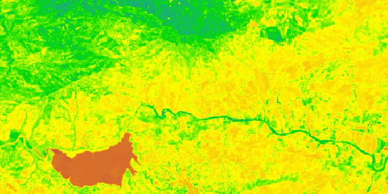
Use map algebra when you need to derive a new surface or category map from one or more input datasets. Common examples include:

creating suitability or risk surfaces from weighted criteria
classifying continuous values into discrete ranges
masking analysis to include only areas that meet a condition
combining intermediate analysis outputs into a final model

Map algebra expressions

In ArcGIS Maps SDK for Qt, you create map algebra expressions with ContinuousFieldFunction, DiscreteFieldFunction, and BooleanFieldFunction objects, then evaluate the final function to produce a new field.

When designing map algebra expressions, it may help to break the logic into intermediate functions rather than composing everything in one statement. This can make complex models easier to read, test, and update.

A common pattern is:

normalize or scale input values so they can be compared consistently
mask out cells that should be excluded from analysis
derive intermediate boolean or discrete categories from thresholds
combine intermediate outputs into the final classified or continuous result

Map algebra operations

The tables below list many of the available operations for each type of field function. Each operation is implemented as a method on the field function class. See the ContinuousFieldFunction, DiscreteFieldFunction, and BooleanFieldFunction for details.

Method	Composes a function that
`ContinuousFieldFunction::add()` `DiscreteFieldFunction::Add()`	Adds, point-wise, another compatible field function or a constant value.
`ContinuousFieldFunction::subtract()` `DiscreteFieldFunction::subtract()`	Subtracts, point-wise, another compatible field function or a constant value.
`ContinuousFieldFunction::multiply()` `DiscreteFieldFunction::multiply()`	Multiplies, point-wise, by another compatible field function or a constant value.
`ContinuousFieldFunction::divide()` `DiscreteFieldFunction::divide()`	Divides, point-wise, by another compatible field function or a constant value.
`ContinuousFieldFunction::remainder()` `DiscreteFieldFunction::remainder()`	Computes the remainder, point-wise, when dividing by another compatible field function or a constant value.
`ContinuousFieldFunction::abs()` `DiscreteFieldFunction::abs()`	Returns the absolute value of the function’s field result across its extent.
`ContinuousFieldFunction::pow()`	Raises each value to a specified exponent, point-wise.
`ContinuousFieldFunction::exp()` `ContinuousFieldFunction::exp10()`	Computes the natural exponential (base $e$) or base-10 exponential of each value, point-wise.
`ContinuousFieldFunction::log()` `ContinuousFieldFunction::log10()`	Computes the natural logarithm or base-10 logarithm of each value, point-wise.
`ContinuousFieldFunction::sqrt()`	Computes the square root of each value, point-wise.
`ContinuousFieldFunction::reciprocal()`	Computes the reciprocal ($1/x$) of each value, point-wise.
`ContinuousFieldFunction::ceil()` `ContinuousFieldFunction::floor()` `ContinuousFieldFunction::round()`	Rounds continuous values up, down, or to the nearest integer across the function’s extent.

Method	Composes a function that
`ContinuousFieldFunction::sin()` `ContinuousFieldFunction::cos()` `ContinuousFieldFunction::tan()`	Computes the sine, cosine, or tangent of the function’s field result across its extent. The result is in radians.
`ContinuousFieldFunction::asin()` `ContinuousFieldFunction::acos()` `ContinuousFieldFunction::atan()`	Computes the arcsine, arccosine, or arctangent of the function’s field result across its extent. The result is in radians.

Method	Composes a function that
`ContinuousFieldFunction::isGreaterThan()` `DiscreteFieldFunction::isGreaterThan()`	Indicates, point-wise, where the function’s field result is greater than another compatible field function or a constant value.
`ContinuousFieldFunction::isGreaterThanOrEqualTo()` `DiscreteFieldFunction::isGreaterThanOrEqualTo()`	Indicates, point-wise, where the function’s field result is greater than or equal to another compatible field function or a constant value.
`ContinuousFieldFunction::isLessThan()` `DiscreteFieldFunction::isLessThan()`	Indicates, point-wise, where the function’s field result is less than another compatible field function or a constant value.
`ContinuousFieldFunction::isLessThanOrEqualTo()` `DiscreteFieldFunction::isLessThanOrEqualTo()`	Indicates, point-wise, where the function’s field result is less than or equal to another compatible field function or a constant value.
`DiscreteFieldFunction::isEqualTo()`	Indicates, point-wise, where the discrete function’s field result is equal to another discrete function or a constant value.
`DiscreteFieldFunction::isNotEqualTo()`	Indicates, point-wise, where the discrete function’s field result is not equal to another discrete function or a constant value.

Method	Composes a function that
`BooleanFieldFunction::logicalAnd()`	Indicates, point-wise, where both boolean function results are true.
`BooleanFieldFunction::logicalOr()`	Indicates, point-wise, where either boolean function result is true.
`BooleanFieldFunction::logicalXor()`	Indicates, point-wise, where exactly one boolean function result is true.
`BooleanFieldFunction::logicalNot()`	Inverts the boolean function result point-wise across its extent.

Method	Composes a function that
`ContinuousFieldFunction::hasData()` `DiscreteFieldFunction::hasData()` `BooleanFieldFunction::hasData()`	Identifies, point-wise, where the function’s field result has data.
`ContinuousFieldFunction::mask()` `DiscreteFieldFunction::mask()` `BooleanFieldFunction::mask()`	Applies a boolean mask so results are retained only where the mask evaluates to true.
`ContinuousFieldFunction::replaceIf()` `DiscreteFieldFunction::replaceIf()` `BooleanFieldFunction::replaceIf()`	Preserves the current result or replaces it with another function result or constant value based on a boolean selection.

Method	Composes a function that
`ContinuousFieldFunction::toDiscreteFieldFunction()` `BooleanFieldFunction::toDiscreteFieldFunction()`	Casts the function’s result to a discrete integer-valued field.
`DiscreteFieldFunction::toContinuousFieldFunction()`	Casts the function’s result to a continuous floating-point field.

Implement a map algebra workflow

You can implement map algebra using a pattern like the following:

Create one or more input fields from input spatial data.

You can load raster data into ContinuousField, DiscreteField, or BooleanField objects. Use API like ContinuousField::createAsync() to create fields from source raster datasets.
Create field functions from the input fields and prepare data for analysis.

Create ContinuousFieldFunction, DiscreteFieldFunction, or BooleanFieldFunction objects from the input fields. Prepare the data for analysis by masking out areas that should be excluded, normalizing values, or applying other transformations to the input fields.
Compose map algebra expressions.

Build expressions from arithmetic, trigonometric, logical, relational, and conditional operations to transform values and produce derived outputs. You can also convert between field types, for example with ContinuousFieldFunction::toDiscreteFieldFunction() and DiscreteFieldFunction::toContinuousFieldFunction().
Evaluate the final function.

Evaluation of an expression is deferred until it is explicitly requested (lazy evaluation). Call ContinuousFieldFunction::evaluateAsync() (or the equivalent evaluate method for the function type you are working with) on the final expression to create the output field.
Visualize and optionally persist the result.

Display continuous results with a StretchRenderer and categorical results with a ColormapRenderer. You can add analyses to an AnalysisOverlay to display results. An AnalysisOverlay allows you to group related analyses and control visibility for all members of the collection. A GeoView can contain many analysis overlays. You can also export output fields for reuse by writing GeoTIFF files, for example with ContinuousField::exportToFilesAsync().

Example

Categorize an elevation raster with map algebra

The following example follows the pattern described above to apply map algebra to an elevation raster and categorize values into classes. The workflow creates a field function expression, evaluates it to produce a result field, and then renders the categories in a map view.

Create a source field from raster data.
Create a ContinuousField from an elevation raster. Create a Map to display the original raster so users can compare inputs and outputs.
Create a field function from the raster field and mask out values at or below sea level.
Create a ContinuousFieldFunction from the ContinuousField of elevation values. Mask out values at or below sea level so that only land areas are categorized in the final output.
Build expressions that create categories of elevation values.
Compose map algebra expressions that use mathematical and relational operations to create categorized output fields based on elevation.
Evaluate the final expression to produce a discrete field of geomorphic categories.
None of the intermediate functions are evaluated until the final expression is evaluated. Call ContinuousFieldFunction::evaluateAsync() to produce a DiscreteField of geomorphic categories.
Render the output categories.
Export the evaluated field if needed, create a RasterLayer from the result, and apply a ColormapRenderer so each category is symbolized with a distinct color.

This pattern can be adapted to many use cases beyond elevation classification, such as vegetation index thresholding, terrain suitability modeling, and multi-criteria risk mapping.