This quick tutorial demonstrates some of the basic capabilities of ArcGIS GeoAnalytics for Microsoft Fabric. The tutorial covers how to enable the library, how to access and manipulate data through DataFrames, as well as an overview of how to use SQL functions, track functions, and analysis tools. Finally, it explains how to visualize and save your results.
Introduction
ArcGIS GeoAnalytics for Microsoft Fabric must be enabled by a tenant administrator before it can be used. As a tenant administrator you can turn on or off the GeoAnalytics for Microsoft Fabric library within the Fabric Runtime by going to Settings > Admin Portal > Tenant settings. When disabled, this library will not be available to use in Spark notebooks or Spark job definitions.
Once GeoAnalytics for Microsoft Fabric is enabled, import and authorize the GeoAnalytics for Microsoft Fabric module and then try out the API by importing the SQL functions with an easy-to-use alias like ST and list the first 20 functions in a notebook cell:
import geoanalytics_fabric
from geoanalytics_fabric.sql import functions as ST
spark.sql("show user functions like 'ST_*'").show()Creating DataFrames
GeoAnalytics for Microsoft Fabric includes a Python API and a Scala API that extend Spark with spatial capabilities. GeoAnalytics for Microsoft Fabric uses Spark DataFrames along with custom geometry data types to represent spatial data. A Spark DataFrame is like a Pandas DataFrame or a table in a relational database but is optimized for distributed queries.
GeoAnalytics for Microsoft Fabric comes with several DataFrame extensions for reading from spatial data sources like shapefiles and feature services, in addition to any data source that Spark supports. When reading from a shapefile, file geodatabase, GeoJSON, GeoParquet or feature service, a geometry column will be created automatically. For other data sources, a geometry column can be created from text or binary columns using GeoAnalytics for Microsoft Fabric functions.
The following example shows how to create a Spark DataFrame from a feature service of USA county boundaries, and then show the column names and types.
import geoanalytics_fabric
df = spark.read.format("feature-service").load("https://services.arcgis.com/P3ePLMYs2RVChkJx/ArcGIS/rest/services/USA_Census_Counties/FeatureServer/0")
df.printSchema()root
|-- OBJECTID: integer (nullable = false)
|-- NAME: string (nullable = true)
|-- STATE_NAME: string (nullable = true)
|-- STATE_ABBR: string (nullable = true)
|-- STATE_FIPS: string (nullable = true)
|-- COUNTY_FIPS: string (nullable = true)
|-- FIPS: string (nullable = true)
|-- POPULATION: integer (nullable = true)
|-- POP_SQMI: double (nullable = true)
|-- SQMI: double (nullable = true)
|-- Shape__Area: double (nullable = true)
|-- Shape__Length: double (nullable = true)
|-- shape: polygon (nullable = true)Learn more about using Spark DataFrames with GeoAnalytics for Microsoft Fabric.
Using functions and tools
GeoAnalytics for Microsoft Fabric includes three core modules for manipulating DataFrames:
geoanalytics contains spatial functions that operate on
columns to do things like create or export geometries, identify spatial
relationships, generate bins, and more. These functions can be called through
Python or Scala functions or by using SQL, similar to Spark SQL functions.
The following example shows how to use a SQL function through Python.
import geoanalytics_fabric.sql.functions as ST
# Calculate the centroid of each county polygon
county_centroids = df.select("Name", ST.centroid("shape"))
# Display the first 5 rows of the result
county_centroids.show(5)+--------------+--------------------+
| Name| ST_Centroid(shape)|
+--------------+--------------------+
|Autauga County|{"x":-86.64274917...|
|Baldwin County|{"x":-87.72434243...|
|Barbour County|{"x":-85.39319698...|
| Bibb County|{"x":-87.12643963...|
| Blount County|{"x":-86.56737098...|
+--------------+--------------------+
only showing top 5 rowsgeoanalytics contains spatial functions for managing and analyzing track data.
Tracks are linestrings that represent the change in an entity's location over time.
These functions can be called through Python or Scala functions or by using SQL, similar to Spark SQL functions.
The following example shows how to use a track function through Python.
from geoanalytics_fabric.tracks import functions as TRK
from geoanalytics_fabric.sql import functions as ST
from pyspark.sql import functions as F
data = [
("LINESTRING M (-117.27 34.05 1633455010, -117.22 33.91 1633456062, -116.96 33.64 1633457132)",),
("LINESTRING M (-116.89 33.96 1633575895, -116.71 34.01 1633576982, -116.66 34.08 1633577061)",),
("LINESTRING M (-116.24 33.88 1633575234, -116.33 34.02 1633576336)",)
]
# Create tracks from WKT
trk_df = spark.createDataFrame(data, ["wkt",]) \
.withColumn("track", ST.line_from_text("wkt", srid=4326))
# Calculate the length of each track and display it
trk_df.select(F.round(TRK.length("track", "miles"), 3).alias("length")).show()+------+
|length|
+------+
|33.947|
|16.507|
|10.947|
+------+geoanalytics contains spatial and spatiotemporal analysis tools that
execute multi-step workflows on entire DataFrames using geometry, time,
and other values. These tools can only be called with their associated
Python classes.
from geoanalytics_fabric.tools import FindSimilarLocations
# Use Find Similar Locations to find counties with population count and density like Alexander County
fsl = FindSimilarLocations() \
.setAnalysisFields("POP_SQMI","POPULATION") \
.setMostOrLeastSimilar("MostSimilar") \
.setNumberOfResults(5) \
.setAppendFields("NAME", "STATE_NAME") \
.run(df.where("NAME = 'Alexander County'"), df.where("NAME != 'Alexander County'"))
# Show the result
fsl.select("simrank", "NAME", "STATE_NAME").filter("NAME is not NULL").sort("simrank").show()+-------+----------------+--------------+
|simrank| NAME| STATE_NAME|
+-------+----------------+--------------+
| 1| Greene County|North Carolina|
| 2|St. James Parish| Louisiana|
| 3| Union County| Tennessee|
| 4| McDuffie County| Georgia|
| 5| Dakota County| Nebraska|
+-------+----------------+--------------+Exploring results
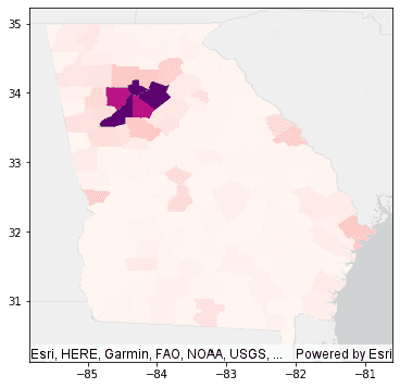
When scripting in a notebook-like environment, GeoAnalytics for Microsoft Fabric supports simple visualization of spatial data with an included plotting API based on matplotlib.
# Plot counties in Georgia and symbolize on population
df.where("STATE_NAME = 'Georgia'").st.plot(cmap_values="POPULATION", cmap="RdPu", figsize=(6,6), basemap="light")
Writing out results
Any DataFrame can be persisted by writing it to a collection of shapefiles, vector tiles, or any data sink supported by Spark.
# Example writing out a DataFrame as a GeoParquet to Microsoft OneLake
df.write.format("geoparquet").save(r"Files/geoanalytics_fabric_examples/python/df_geoparquet_output")Related content
What's next?
To get started, learn about using and loading data into DataFrames, running analysis tools and functions, and visualizing results through the available guides and tutorials: