Introduction
This guide demonstrates the use of deep learning capabilities in ArcGIS to perform feature categorization. Specifically, we are going to perform automated damage assessment of homes after the devastating Woolsey fires. This is a critical task in damage claim processing, and using deep learning can speed up the process and make it more efficient. The workflow consists of three major steps: (1) extract training data, (2) train a deep learning feature classifier model, (3) make inference using the model.

Figure 1. Feature classification example
Part 1 - export training data for deep learning
To export training data for feature categorization, we need two input data:
- A input raster that contains the spectral bands,
- A feature class that defines the location (e.g. outline or bounding box) and label of each building.
Import ArcGIS API for Python and get connected to your GIS
from arcgis import GISgis = GIS("home")Prepare data that will be used for training data export
First, let's get the feature class that defines the location and label of each building.
building_label = gis.content.search("damage_labelselection_Buffer_100", item_type='Feature Layer Collection')[0]
building_label
Now let's get input raster that contains the spectral bands.
gis2 = GIS("https://ivt.maps.arcgis.com")input_raster_layer = gis2.content.search("111318_USAA_W_Malibu")[0]
input_raster_layer
Specify a folder name in raster store that will be used to store our training data
from arcgis.raster import analytics

ds = analytics.get_datastores(gis=gis)
ds
<DatastoreManager for https://datascienceadv.esri.com/server/admin>
ds.search()[<Datastore title:"/nosqlDatabases/AGSDataStore_bigdata_bds_4c9tuc3o" type:"nosql">, <Datastore title:"/nosqlDatabases/AGSDataStore_nosqldb_tcs_l6mh5mhm" type:"nosql">, <Datastore title:"/enterpriseDatabases/AGSDataStore_ds_b6108wk9" type:"egdb">, <Datastore title:"/rasterStores/LocalRasterStore" type:"rasterStore">]
rasterstore = ds.get("/rasterStores/LocalRasterStore")
rasterstore
<Datastore title:"/rasterStores/LocalRasterStore" type:"rasterStore">
samplefolder = "feature_classifier_sample"
samplefolder
'feature_classifier_sample'
Export training data using arcgis.learn
Now ready to export training data using the export_training_data() method in arcgis.learn module. In addtion to feature class, raster layer, and output folder, we also need to specify a few other parameters such as tile_size (size of the image chips), stride_size (distance to move each time when creating the next image chip), chip_format (TIFF, PNG, or JPEG), metadata_format (how we are going to store those training labels). Note that unlike Unet and object detection, the metadata is set to be Labeled_Tiles here. More detail can be found here.
Depending on the size of your data, tile and stride size, and computing resources, this operation can take a while. In our experiments, this took 15mins~2hrs. Also, do not re-run it if you already run it once unless you would like to update the setting.
import arcgis
from arcgis import learn
arcgis.env.verbose = True
export = learn.export_training_data(input_raster=input_raster_layer,
output_location=samplefolder,
input_class_data=building_label,
classvalue_field = "classValue",
chip_format="PNG",
tile_size={"x":600,"y":600},
stride_size={"x":0,"y":0},
metadata_format="Labeled_Tiles",
context={"startIndex": 0, "exportAllTiles": False, "cellSize": 0.1},
gis = gis)Part 2 - model training
If you've already done part 1, you should already have the training chips. Please change the path to your own export training data folder that contains "images" and "labels" folder.
from arcgis.learn import prepare_data, FeatureClassifierdata_path = r'to_your_data_folder'
data = prepare_data(data_path, {1:'Damaged', 0:'Undamaged'}, chip_size=600, batch_size=16)Visualize training data
To get a sense of what the training data looks like, arcgis.learn.show_batch() method randomly picks a few training chips and visualize them.
data.show_batch()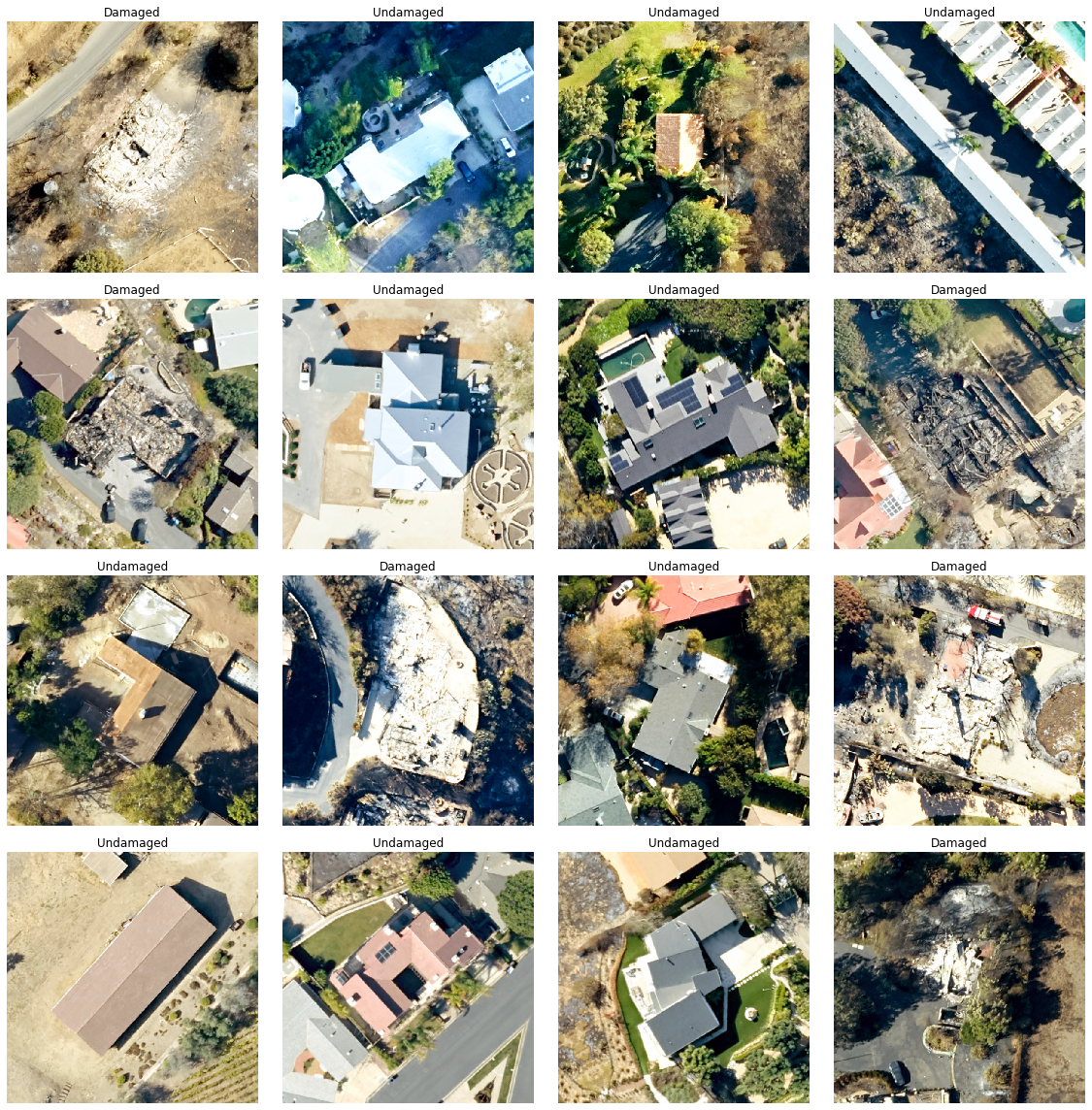
Load model architecture
Now the building classification problem has become a standard image classfication problem. By default arcgis.learn uses Resnet34 as its backbone model followed by a softmax layer.

Figure 2. Resnet34 architecture [1]
model = FeatureClassifier(data)Train a model through learning rate tuning and transfer learning
Learning rate is one of the most important hyperparameters in model training. Here we explore a range of learning rates to guide us to choose the best one.
# The users can visualize the learning rate of the model with comparative loss. This case - loss rate decreases, so we are detecting more n more objects as it learns more
model.lr_find()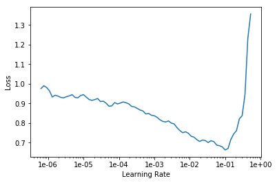
Based on the learning rate plot above, we can see that the loss going down most dramatically at 1e-2. Therefore, we set learning rate to be to 1e-2. Let's start with 10 epochs for the sake of time.
model.fit(epochs=10, lr=1e-2)| epoch | train_loss | valid_loss | accuracy |
|---|---|---|---|
| 1 | 0.188588 | 0.091087 | 0.976510 |
| 2 | 0.185616 | 0.066837 | 0.969799 |
| 3 | 0.195557 | 0.174460 | 0.919463 |
| 4 | 0.126604 | 0.049342 | 0.983221 |
| 5 | 0.131944 | 0.051884 | 0.984899 |
| 6 | 0.112607 | 0.052149 | 0.978188 |
| 7 | 0.101093 | 0.025041 | 0.996644 |
| 8 | 0.074809 | 0.031996 | 0.986577 |
| 9 | 0.058637 | 0.025428 | 0.989933 |
| 10 | 0.055728 | 0.023803 | 0.991611 |
Visualize classification results in validation set
Now we have the model, let's look at how the model performs.
model.show_results(rows=4)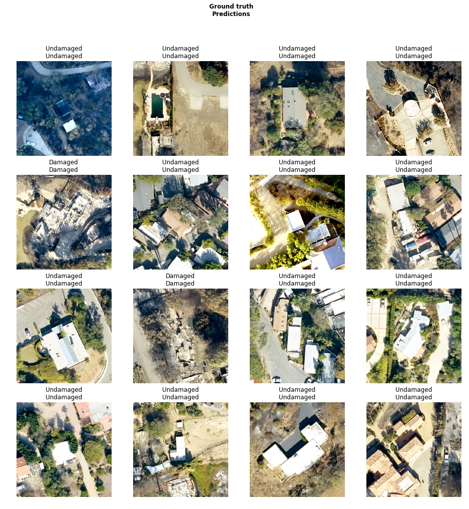
As we can see, with only 10 epochs, we are already seeing reasonable results. Further improvment can be acheived through more sophisticated hyperparameter tuning. Let's save the model for further training or inference later. The model should be saved into a models folder in your folder. By default, it will be saved into your data_path that you specified in the very beginning of this notebook.
model.save('model-10')WindowsPath('D:/feature_classify_folder_100m_buffer/models/model-10')Part 3 - inference
Now we have the model ready, let's apply the model to a new feature class with a few new buildings and see how it performs.
item = gis.content.search("inference_layer", item_type='Feature Layer Collection')[0]
item
Unlike object detection and pixel-based classification, we can use categorize_features() directly without publishing or installing the model. There a few import parameters here.
- raster: a raster data that provides spectral information for inference. Ideally, it should be the same or similar to the raster you used to train the model.
- class_value_field: Output field to be added in the layer, containing class value of predictions.
- class_name_field: Output field to be added in the layer, containing class name of predictions.
- confidence_field: Output column name to be added in the layer which contains the confidence score (optional).
- overwrite: If set to True the output fields will be overwritten by new values.
model = FeatureClassifier.from_model(r'path_to_your_model')model.categorize_features(feature_layer=item.layers[0],
raster=input_raster_layer.url,
class_value_field='class_val1',
class_name_field='prediction1',
confidence_field="confidence1",
cell_size=.1,
batch_size=16,
overwrite=True
) We can load the inference layer into a spatially enabled dataframe to examine the inference result.
import pandas as pd
from arcgis.features import GeoAccessor, GeoSeriesAccessor

sdf = pd.DataFrame.spatial.from_layer(item.layers[0])
sdf[['bld_id', 'usetype', 'ground_truth','prediction1', 'class_val1', 'confidence1']].head(10)| bld_id | usetype | ground_truth | prediction1 | class_val1 | confidence1 | |
|---|---|---|---|---|---|---|
| 0 | 312778833124 | Residential | DAMAGED | Damaged | 1 | 408.642944 |
| 1 | 312745833781 | Residential | Undamaged | Undamaged | 0 | 376.614685 |
| 2 | 313750833138 | Residential | Undamaged | Undamaged | 0 | 322.914398 |
| 3 | 313308832529 | Residential | Undamaged | Undamaged | 0 | 448.014923 |
| 4 | 313868832780 | Residential | Undamaged | Undamaged | 0 | 313.009277 |
| 5 | 313085833616 | Residential | DAMAGED | Damaged | 1 | 308.200592 |
| 6 | 313200832345 | Residential | DAMAGED | Damaged | 1 | 354.850830 |
| 7 | 313100832645 | Residential | DAMAGED | Damaged | 1 | 319.919189 |
| 8 | 313462833517 | Residential | Undamaged | Undamaged | 0 | 407.920685 |
| 9 | 313189833045 | Residential | Undamaged | Undamaged | 0 | 548.331055 |
As we can see, all sample buildings are classified correctly with high confidence.
Reference
[1] Ruiz Pablo, Understanding and Visualizing ResNets, https://towardsdatascience.com/understanding-and-visualizing-resnets-442284831be8, Accessed 2 September 2019.