Deep learning models 'learn' by looking at several examples of imagery and the expected outputs. In the case of object detection, this requires imagery as well as known or labelled locations of objects that the model can learn from. With the ArcGIS platform, these datasets are represented as layers, and are available in GIS. In the workflow below, we will be training a model to identify well pads from Planet imagery.
Prerequisites
- Please refer to the prerequisites section in our guide for more information. This sample demonstrates how to export training data and model inference using ArcGIS Image Server. Alternatively, this can be done using ArcGIS Pro as well.
- If you have already exported training samples using ArcGIS Pro, you can jump straight to the training section. The saved model can also be imported into ArcGIS Pro directly.
The code below connects to our GIS and accesses the known well pad locations and the imagery, in this case provided by Planet:
from arcgis.gis import GIS
from arcgis.raster.functions import extract_band
from arcgis.learn import export_training_data

gis = GIS("home")
# layers we need - The input to generate training samples and the imagery
well_pads = gis.content.get('ae6f1c62027c42b8a88c4cf5deb86bbf') # Well pads layer
well_pads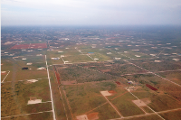
# Weekly mosaics provided by Planet
planet_mosaic_item = gis.content.search("PlanetGlobalMosaics")[0]
planet_mosaic_item
Export Training Samples
The export_training_data() method generates training samples for training deep learning models, given the input imagery, along with labelled vector data or classified images. Deep learning training samples are small sub images, called image chips, and contain the feature or class of interest. This tool creates folders containing image chips for training the model, labels and metadata files and stores them in the raster store of your enterprise GIS. The image chips are often small (e.g. 256x256), unless the training sample size is large. These training samples support model training workflows using the arcgis.learn package as well as by third-party deep learning libraries, such as TensorFlow or PyTorch. The supported models in arcgis.learn accept the PASCAL_VOC_rectangles format for object detection models, which is a standardized image dataset for object class recognition. The label files are XML files containing information about image name, class value, and bounding boxes.
In order to take advantage of pretrained models that have been trained on large image collections (e.g. ImageNet), we have to pick 3 bands from a multispectral imagery, as those pretrained models are trained with images that have only 3 RGB channels. The extract_bands() method can be used to specify which 3 bands should be extracted for fine tuning the models:
planet_mosaic_data = extract_band(planet_mosaic_item.layers[0], [1,2,3])We recommend exporting image chips with a larger size than that used for training the models. This allows arcgis.learn to perform random center cropping as part of its default data augmentation and makes the model see a different sub-area of each chip when training, leading to better generalization and avoiding overfitting to the training data. By default, a chip size of 448 x 448 pixels works well, but this can be adjusted based on the amount of context you wish to provide to the model, as well as the amount of GPU memory available.
chips = export_training_data(input_raster=planet_mosaic_data,
                             input_class_data=well_pads,
                             chip_format="PNG",
                             tile_size={"x":448,"y":448},
                             stride_size={"x":224,"y":224},
                             metadata_format="PASCAL_VOC_rectangles",
                             classvalue_field='pad_type',
                             buffer_radius=75,
                             output_location="/rasterStores/rasterstorename/wellpaddata")
Data Preparation
Data preparation can be a time consuming process that typically involves splitting the data into training and validation sets, applying various data augmentation techniques, creating the necessary data structures for loading data into the model, managing memory by using the appropriately sized mini-batches of data, and so on. The prepare_data() method can directly read the training samples exported by ArcGIS and automate the entire process.
By default, prepare_data() uses a default set of transforms for data augmentation that work well for satellite imagery. These transforms randomly rotate, scale and flip the images so the model sees a different image each time. Alternatively, users can compose their own transforms using fast.ai transforms for the specific data augmentations they wish to perform.
from arcgis.learn import prepare_data

data = prepare_data('/rasterStores/rasterstorename/wellpaddata', {1: '  Pad'})
The show_batch() method can be used to visualize the exported training samples, along with labels, after data augmentation transformations have been applied.
data.show_batch()
Model Training
arcgis.learn includes support for training deep learning models for object detection.
The models in arcgis.learn are based upon pretrained Convolutional Neural Networks (CNNs, or in short, convnets) that have been trained on millions of common images such as those in the ImageNet dataset. The intuition of a CNN is that it uses a hierarchy of layers: the earlier layers learn to identify simple features like edges and blobs, the middle layers combine these primitive features to identify corners and object parts, and the later layers combine the inputs from these in unique ways to grasp what the whole image is about. The final layer in a typical convnet is a fully connected layer that looks at all the extracted features and essentially computes a weighted sum of these to determine a probability of each object class (whether its an image of a cat or a dog, etc.).
A convnet trained on a huge corpus of images such as ImageNet is thus considered as a ready-to-use feature extractor. In practice, we could replace the last layer of these convnets with something else that uses those features for other useful tasks (e.g. object detection and pixel classification), which is also called transfer learning. The advantage of transfer learning is that we now don't need as much data to train an excellent model.
The arcgis.learn module is based on PyTorch and fast.ai and enables fine-tuning of pretrained torchvision models on satellite imagery. The arcgis.learn models leverages fast.ai's learning rate finder and one-cycle learning, and allows for much faster training and removes guesswork in picking hyperparameters.
arcgis.learn provides the SingleShotDetector (SSD) model for object detection tasks, which is based on a pretrained convnet, like ResNet that acts as the 'backbone'. More details about SSD can be found here.
Train SingleShotDetector Model
Since the image chips visualized in the section above indicate that most well pads are roughly of the same size and square in shape, we can keep an aspect ratio of 1:1 and zoom scale of 1. This will help simplify the model and make it easier to train. Also, since the size of well pads in the image chips is such that approximately nine could fit side by side, we can keep a grid size of 9.
from arcgis.learn import SingleShotDetector

ssd = SingleShotDetector(data, grids=[9], zooms=[1.0], ratios=[[1.0, 1.0]])
Find the efficient learning rate
Now, once a model architecture is defined we can start to train it. This process involves setting a good learning rate.
Choosing a very small learning rate leads to very slow training of the model, while selecting an extremely high rate can 'overshoot' the minima where the loss (or error rate) is lowest, and prevent the model from converging.
arcgis.learn includes learning rate finder, and is accessible through the model's lr_find() method, that can automatically select an optimum learning rate, without requiring repeated experiments.
# The users can visualize the learning rate of the model with comparative loss.
ssd.lr_find()
The above function returns 0.001 as the learning rate.
Train the model
As discussed earlier, the idea of transfer learning is to fine-tune earlier layers of the pretrained model and focus on training the newly added layers, meaning we need two different learning rates to better fit the model. We have already selected a good learning rate to train the later layers above (i.e. 0.02). An empirical value of lower learning rate for fine-tuning the earlier layers is usually one tenth of the higher rate. We choose 0.001 to be more careful not to disturb the weights of the pretrained backbone by too much. It can be adjusted depending upon how different the imagery is from natural images on which the backbone network is trained.
Training the network is an iterative process. We can train the model using its fit() method until the validation loss (or error rate) continues to go down with each training pass (also known as epoch). This is indicative of the model learning the task.
Optionally, if we pass early_stopping=True as a parameter in fit() method, it stops training the model if validation loss doesn't decrease for 5 consecutive epochs. Moreover, checkpoint=True parameter saves the best model based on validation loss during training.
Note: You may also choose not to pass lr parameter. The method automatically calls lr_find() function to find an optimum learning rate if lr parameter is not set.
# here we are training the model for 10 epochs
ssd.fit(10, lr=0.001)| epoch | train_loss | valid_loss |
|---|---|---|
| 1 | 1743.360840 | 759.151855 |
| 2 | 1700.622559 | 763.675842 |
| 3 | 1691.474487 | 733.454163 |
| 4 | 1705.710205 | 736.463928 |
| 5 | 1715.943115 | 731.263000 |
| 6 | 1718.531738 | 734.463257 |
| 7 | 1705.809692 | 736.284851 |
| 8 | 1706.338623 | 738.023926 |
| 9 | 1707.944458 | 724.500916 |
| 10 | 1701.971069 | 727.411438 |
As each epoch progresses, the loss (error rate, that we are trying to minimize) for the training data and the validation set are reported. In the table above we can see the losses going down for both the training and validation datasets, indicating that the model is learning to recognize the well pads. We continue training the model for several iterations till we observe the validation loss going up. That indicates that the model is starting to overfit to the training data, and is not generalizing well enough for the validation data. When that happens, we can either add more data (or data augmentations), or increase regularization by increasing the dropout parameter in the SingleShotDetector model, or reduce the model complexity.
Unfreezing the backbone and fine-tuning
By default, the earlier layers of all the vision models (i.e. the backbone or encoder) are frozen and their weights are not updated when the model is being trained. This allows the model to take advantage of the (ImageNet) pretrained weights for training the 'head' of the network. In case of text models, the backbone is unfrozen (trainable) by default.
Once the later layers have been sufficiently trained, the earlier layers are unfrozen (by calling unfreeze()) and and fine-tuned to the nuances of the particular satellite imagery. Using satellite imagery rather than photos of everyday objects (from ImageNet) that the backbone was initially trained on, helps to improve model performance and accuracy.
The learning rate finder can be used to identify the optimum learning rate between the different training phases of the model. Please note that this step is optional. If we don't call unfreeze(), the lower learning rate we specified in the fit() won't be used.
Visualize results
The results of how well the model has learnt can be visually observed using the model's show_results() method. The ground truth is shown in the left column and the corresponding predictions from the model on the right. As we can see below, the model has learnt to detect well pads fairly well. In some cases, it is even able to detect the well pads that are missing in the ground truth data (due to inaccuracies in labelling or the records).
ssd.show_results(rows=25, thresh=0.05)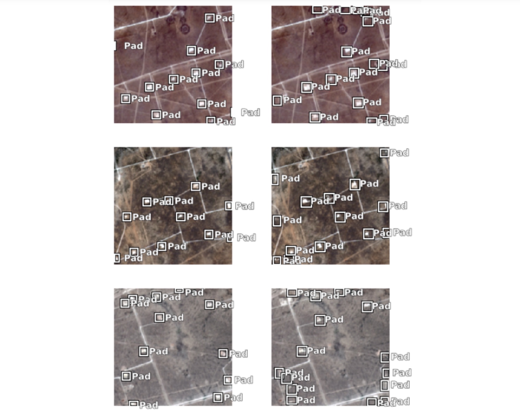
Save and load trained models
Once you are satisfied with the model, you can save it using the save() method. This creates an Esri Model Definition (EMD file) that can be used for inferencing in ArcGIS Pro as well as a Deep Learning Package (DLPK zip) that can be deployed to ArcGIS Enterprise for distributed inferencing across a large geographical area using raster analytics. Saved models can also be loaded back using the load() method, for futher fine tuning.
save() method takes in additional argument framework which defaults to PyTorch.
# save the trained model
ssd.save('wellpad_planet_model', publish=True)
Once a model has been trained, it can be added to ArcGIS Enterprise as a deep learning package by passing publish=True parameter.
Model management
model_package = gis.content.get('id=32cb1df2834943f7a6ff3ab461aa9352')
model_packageThe arcgis.learn module includes the install_model() method to install the uploaded model package (*.dlpk) to the raster analytics server.
Optionally after inferencing the necessary information from the imagery using the model, the model can be uninstalled using uninstall_model(). The deployed models on an Image Server can be queried using the list_models() method. The uploaded model package is installed automatically on first use as well. Here we are querying specific settings of the deep learning model using the model object:
from arcgis.learn import Model

detect_objects_model = Model(model_package)
detect_objects_model.install()
detect_objects_model.query_info()
{'Framework': 'arcgis.learn.models._inferencing',
'ModelType': 'ObjectDetection',
'ParameterInfo': [{'name': 'raster',
'dataType': 'raster',
'required': '1',
'displayName': 'Raster',
'description': 'Input Raster'},
{'name': 'model',
'dataType': 'string',
'required': '1',
'displayName': 'Input Model Definition (EMD) File',
'description': 'Input model definition (EMD) JSON file'},
{'name': 'device',
'dataType': 'numeric',
'required': '0',
'displayName': 'Device ID',
'description': 'Device ID'},
{'name': 'padding',
'dataType': 'numeric',
'value': '0',
'required': '0',
'displayName': 'Padding',
'description': 'Padding'},
{'name': 'threshold',
'dataType': 'numeric',
'value': '0.5',
'required': '0',
'displayName': 'Confidence Score Threshold [0.0, 1.0]',
'description': 'Confidence score threshold value [0.0, 1.0]'},
{'name': 'nms_overlap',
'dataType': 'numeric',
'value': '0.1',
'required': '0',
'displayName': 'NMS Overlap',
'description': 'Maximum allowed overlap within each chip'},
{'name': 'batch_size',
'dataType': 'numeric',
'required': '0',
'value': '64',
'displayName': 'Batch Size',
'description': 'Batch Size'}]}Here we can see that threshold and nms_overlap are model arguments with default value of 0.5 and 0.1 respectively. These values may be changed in the detect_objects() function call.
Model inference
The detect_objects() function can be used to generate feature layers that contains bounding box around the detected objects in the imagery data using the specified deep learning model.
Note that the deep learning library dependencies needs to be installed separately, in addition on the image server.
Refer to the "Install deep learning dependencies of arcgis.learn module" section on this page for detailed documentation on installation of these dependencies.
The code below shows how we can use distributed raster analytics to automate the detection of well pad for different dates, across a large geographical area and create a feature layer of well pad detections that can be used for further analysis within ArcGIS.
context = {'cellSize': 10,
           'processorType':'GPU',
           'extent':{'xmin': -11392183,
                     'ymin': 3764168,
                     'xmax': -11385824,
                     'ymax': 3766079, 'spatialReference': {'latestWkid': 3857, 'wkid': 102100}}}
from arcgis.learn import detect_objects
detected_pads = []
input_layers = []
for i in range (3, 13, 2):
input_layers.append(planet_mosaic_data.filter_by('Date='+str(i)))
for i in range(0, len(input_layers)):
detected_pads.append(detect_objects(input_raster=input_layers[i],
model=detect_objects_model,
output_name="Well_Pad_Detection_Planet_items_2501_"+str(i),
context=context,
gis=gis))Visualize results
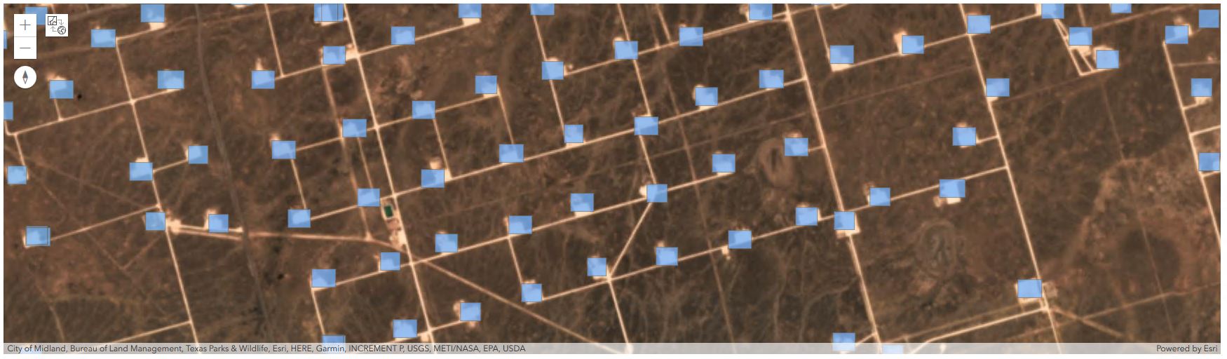
Finally, we can visualize the results using the map widget using the Python API to verify if they are as expected.
web_map = gis.content.search("title: Well Pad Detection 4 AND owner:portaladmin",item_type="Web Map")[0]
map_widget = gis.map(web_map)


map_widget.extent = {'spatialReference': {'latestWkid': 3857, 'wkid': 102100},
 'xmin': -11397184.938845266,
 'ymin': 3761693.7641860787,
 'xmax': -11388891.521276105,
 'ymax': 3764082.4213200537}

map_widget.zoom = 15
map_widget