- 🔬 Data Science
- 🥠 Deep Learning and Pixel Classification
Introduction
In this notebook, we will use 3 different geo-morphological characteristics derived from a 5 m resolution DEM in one of the watersheds of Alaska to extract streams. These 3 characteristics are Topographic position index derived from 3 cells, Geomorphon landform, and topographic wetness index.
We created a composite out of these 3 characteristic rasters and used Export raster tool to convert scale the pixels values to 8 bit unsigned. Subsequently, the images are exported as "Classified Tiles" to train a Multi-Task Road Extractor model provided by ArcGIS API for Python for extracting the streams.
Before proceeding through this notebook, it is advised to go through the API Reference for Multi-Task Road Extractor. It will help in understanding the Multi-Task Road Extractor's workflow in detail.
Necessary imports
import os
import zipfile
from pathlib import Path

from arcgis.gis import GIS
from arcgis.learn import prepare_data, MultiTaskRoadExtractor, ConnectNet
Connect to your GIS
gis = GIS("home")Get the data for analysis
Here is the composite with 3 bands representing the 3 geo-morphological characteristics namely Topographic position index, Geomorphon landform, and Topographic wetness index.
composite_raster = gis.content.get('6323857007ec4500bdc4ed203e19e608')
composite_raster
BeaverCreek_Flowlines = gis.content.get('53c2c22e12dc455aac821b3d7deb60b4')
BeaverCreek_Flowlines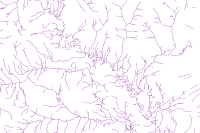
Export training data
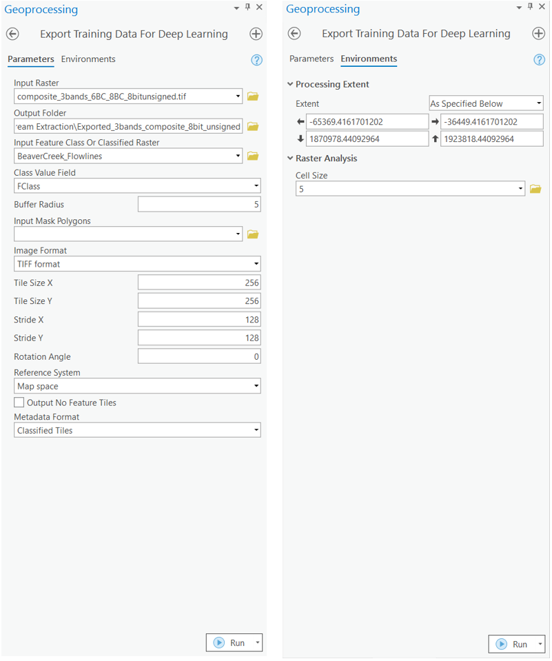
Export training data using 'Export Training data for deep learning' tool, click here for detailed documentation:
- Set 'composite_3bands_6BC_8BC_8bitunsigned' as
Input Raster. - Set a location where you want to export the training data in
Output Folderparameter, it can be an existing folder or the tool will create that for you. - Set the 'BeaverCreek_Flowlines' as input to the
Input Feature Class Or Classified Rasterparameter. - Set
Class Field Valueas 'FClass'. - Set
Image Formatas 'TIFF format' Tile Size X&Tile Size Ycan be set to 256.Stride X&Stride Ycan be set to 128.- Select 'Classified Tiles' as the
Meta Data Format. - In 'Environments' tab set an optimum
Cell Size. For this example, as we have performing the analysis on the geo-morphological characteristics with 5 m resolution, so, we used '5' as the cell size.
arcpy.ia.ExportTrainingDataForDeepLearning("composite_3bands_6BC_8BC_8bitunsigned.tif", r"D:\Stream Extraction\Exported_3bands_composite_8bit_unsigned", "BeaverCreek_Flowlines", "TIFF", 256, 256, 128, 128, "ONLY_TILES_WITH_FEATURES", "Classified_Tiles", 0, "FClass", 5, None, 0, "MAP_SPACE", "PROCESS_AS_MOSAICKED_IMAGE", "NO_BLACKEN", "FIXED_SIZE")
Alternatively, we have provided a subset of training data containing a few samples. You can use the data directly to run the experiments.
training_data = gis.content.get('3a95fd7a25d54898bddabf1989eea87d')
training_data
filepath = training_data.download(file_name=training_data.name)with zipfile.ZipFile(filepath, 'r') as zip_ref:
zip_ref.extractall(Path(filepath).parent)output_path = Path(os.path.join(os.path.splitext(filepath)[0]))Prepare data
We will specify the path to our training data and a few hyperparameters.
path: path of the folder containing training data.batch_size: Number of images your model will train on each step inside an epoch, it directly depends on the memory of your graphic card. 8 worked for us on a 11GB GPU.
data = prepare_data(output_path, chip_size=512, batch_size=4)Visualize a few samples from your training data
To get a sense of what the training data looks like, arcgis.learn.show_batch() method randomly picks a few training chips and visualizes them.
rows: number of rows we want to see the results for.
data.show_batch()
Train the model
Load model architecture
arcgis.learn provides the MultiTaskRoadExtractor model for classifying linear features, which is based on multi-task learning mechanism. More details about multi-task learning can be found here.
model = ConnectNet(data, mtl_model="hourglass")Find an optimal learning rate
Learning rate is one of the most important hyperparameters in model training. Here, we explore a range of learning rate to guide us to choose the best one. We will use the lr_find() method to find an optimum learning rate at which we can train a robust model.
lr=model.lr_find()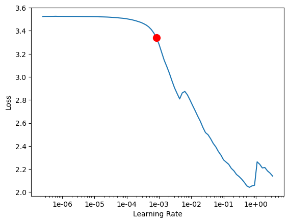
Fit the model
To train the model, we use the fit() method. To start, we will train our model for 50 epochs. Epoch defines how many times model is exposed to entire training set. We have passes three parameters to fit() method:
epochs: Number of cycles of training on the data.lr: Learning rate to be used for training the model.wd: Weight decay to be used.
model.fit(50, lr)| epoch | train_loss | valid_loss | accuracy | miou | dice | time |
|---|---|---|---|---|---|---|
| 0 | 0.632394 | 0.622243 | 0.831117 | 0.415558 | 0.000000 | 09:31 |
| 1 | 0.523310 | 0.540622 | 0.921272 | 0.767462 | 0.732915 | 09:27 |
| 2 | 0.460495 | 0.477187 | 0.933677 | 0.801455 | 0.773366 | 09:31 |
| 3 | 0.367851 | 0.450820 | 0.920820 | 0.781137 | 0.762663 | 09:45 |
| 4 | 0.332831 | 0.402109 | 0.934246 | 0.798507 | 0.768905 | 09:28 |
| 5 | 0.310377 | 0.388170 | 0.934500 | 0.810421 | 0.787407 | 09:25 |
| 6 | 0.302640 | 0.525472 | 0.903933 | 0.752356 | 0.736639 | 09:11 |
| 7 | 0.287657 | 0.379396 | 0.937387 | 0.815219 | 0.794576 | 08:51 |
| 8 | 0.277436 | 0.321924 | 0.952717 | 0.848544 | 0.826755 | 09:08 |
| 9 | 0.255621 | 0.310445 | 0.957915 | 0.860929 | 0.826572 | 09:28 |
| 10 | 0.239402 | 0.321138 | 0.950927 | 0.849954 | 0.834631 | 09:27 |
| 11 | 0.220864 | 0.304691 | 0.956517 | 0.861722 | 0.845410 | 09:26 |
| 12 | 0.207121 | 0.257350 | 0.966467 | 0.887069 | 0.864943 | 09:29 |
| 13 | 0.202419 | 0.262285 | 0.965310 | 0.882947 | 0.865285 | 09:25 |
| 14 | 0.176618 | 0.231487 | 0.971649 | 0.902508 | 0.880668 | 09:25 |
| 15 | 0.168874 | 0.216452 | 0.972327 | 0.905584 | 0.888963 | 09:27 |
| 16 | 0.136014 | 0.188540 | 0.979811 | 0.930707 | 0.917923 | 09:27 |
| 17 | 0.129512 | 0.176698 | 0.981729 | 0.936637 | 0.919920 | 09:27 |
| 18 | 0.117116 | 0.210895 | 0.974122 | 0.913574 | 0.907675 | 09:27 |
| 19 | 0.108324 | 0.186383 | 0.980826 | 0.933778 | 0.927348 | 09:29 |
| 20 | 0.097489 | 0.164423 | 0.985538 | 0.950104 | 0.945752 | 09:27 |
| 21 | 0.085404 | 0.152534 | 0.986984 | 0.954966 | 0.949059 | 09:26 |
| 22 | 0.083308 | 0.160948 | 0.985477 | 0.949354 | 0.941757 | 09:27 |
| 23 | 0.076346 | 0.187536 | 0.978523 | 0.927657 | 0.917851 | 09:29 |
| 24 | 0.070911 | 0.159757 | 0.985682 | 0.950238 | 0.938936 | 09:27 |
| 25 | 0.065770 | 0.133059 | 0.990027 | 0.964982 | 0.959355 | 09:02 |
| 26 | 0.061106 | 0.156357 | 0.988830 | 0.960668 | 0.956349 | 08:50 |
| 27 | 0.053245 | 0.139489 | 0.991672 | 0.970816 | 0.968669 | 09:22 |
| 28 | 0.048812 | 0.135724 | 0.992220 | 0.972749 | 0.970554 | 09:27 |
| 29 | 0.046171 | 0.133197 | 0.992103 | 0.972314 | 0.969314 | 09:27 |
| 30 | 0.042203 | 0.128438 | 0.992629 | 0.974309 | 0.972082 | 09:28 |
| 31 | 0.038529 | 0.137634 | 0.992753 | 0.974585 | 0.973580 | 09:30 |
| 32 | 0.036983 | 0.133612 | 0.993040 | 0.975796 | 0.973621 | 09:31 |
| 33 | 0.032619 | 0.132574 | 0.993444 | 0.977010 | 0.974591 | 09:31 |
| 34 | 0.029943 | 0.136561 | 0.993848 | 0.978449 | 0.976824 | 09:29 |
| 35 | 0.028512 | 0.138760 | 0.994182 | 0.979601 | 0.978411 | 08:41 |
| 36 | 0.026747 | 0.141370 | 0.994071 | 0.979139 | 0.977301 | 09:35 |
| 37 | 0.023180 | 0.144617 | 0.994551 | 0.980824 | 0.978298 | 09:39 |
| 38 | 0.021591 | 0.145519 | 0.994738 | 0.981471 | 0.978221 | 09:30 |
| 39 | 0.020423 | 0.147358 | 0.994983 | 0.982369 | 0.979086 | 09:29 |
| 40 | 0.018053 | 0.158130 | 0.995013 | 0.982494 | 0.979906 | 09:28 |
| 41 | 0.016260 | 0.166778 | 0.995187 | 0.983094 | 0.979154 | 09:25 |
| 42 | 0.015209 | 0.172065 | 0.995374 | 0.983758 | 0.981081 | 09:33 |
| 43 | 0.013977 | 0.178109 | 0.995418 | 0.983915 | 0.981957 | 09:35 |
| 44 | 0.012951 | 0.184526 | 0.995508 | 0.984235 | 0.982004 | 09:22 |
| 45 | 0.012069 | 0.192115 | 0.995561 | 0.984430 | 0.981954 | 08:58 |
| 46 | 0.011576 | 0.196924 | 0.995588 | 0.984529 | 0.981835 | 09:14 |
| 47 | 0.011295 | 0.199699 | 0.995618 | 0.984635 | 0.981966 | 09:31 |
| 48 | 0.011038 | 0.201063 | 0.995629 | 0.984670 | 0.981961 | 09:28 |
| 49 | 0.010929 | 0.201135 | 0.995637 | 0.984702 | 0.982025 | 09:31 |
As you can see, both the losses (valid_loss and train_loss) started from a higher value and ended up to a lower value, that tells our model has learnt well. Let us do an accuracy assessment to validate our observation.
Accuracy Assessment
We can compute the mIOU (Mean Intersection Over Union) for the model we just trained in order to do the accuracy assessment. We can compute the mIOU by calling model.mIOU. It takes the following parameters:
mean: If False returns class-wise mean IOU, otherwise returns mean IOU of all classes combined.
model.mIOU(){'0': 0.9946838165542006, 1: 0.9746457531148588}The model has a mean IOU of 0.97 which proves that the model has learnt well. Let us now see it's results on validation set.
Visualize results in validation set
The code below will pick a few random samples and show us ground truth and respective model predictions side by side. This allows us to validate the results of your model in the notebook itself. Once satisfied we can save the model and use it further in our workflow. The model.show_results() method can be used to display the detected streams.
model.show_results(rows=4)
Save the model
We would now save the model which we just trained as a 'Deep Learning Package' or '.dlpk' format. Deep Learning package is the standard format used to deploy deep learning models on the ArcGIS platform.
We will use the save() method to save the model and by default it will be saved to a folder 'models' inside our training data folder itself.
model.save('stream_ext_50e_2024', overwrite=True, publish=True, gis=gis)Published DLPK Item Id: 99d8629d8ae541209efae8c41393136e
WindowsPath('~/AppData/Local/Temp/streams_extraction_using_connectnet/models/stream_ext_50e_2024')Model inference
The saved model can be used to classify streams using the Classify Pixels Using Deep Learning tool available in ArcGIS Pro, or ArcGIS Enterprise.

arcpy.ia.ClassifyPixelsUsingDeepLearning("composite_3bands_6BC_8BC_8bitunsigned.tif", r"D:/stream_ext_20e/stream_ext_20e.dlpk", "padding 64;batch_size 4;predict_background True;return_probability_raster False;threshold 0.5", "PROCESS_AS_MOSAICKED_IMAGE", None); out_classified_raster.save(r"\Documents\ArcGIS\Packages\Stream Extraction demo_9ee52d\p20\stream_identification.gdb\detected_streams")
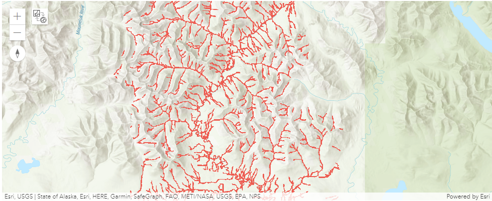
The output of the model is a layer of detected streams which is shown below:
extracted_streams = gis.content.get('3cc376c1bed7428ba50bdf768d28a735')
extracted_streams
map1 = gis.map()
map1.content.add(extracted_streams)
map1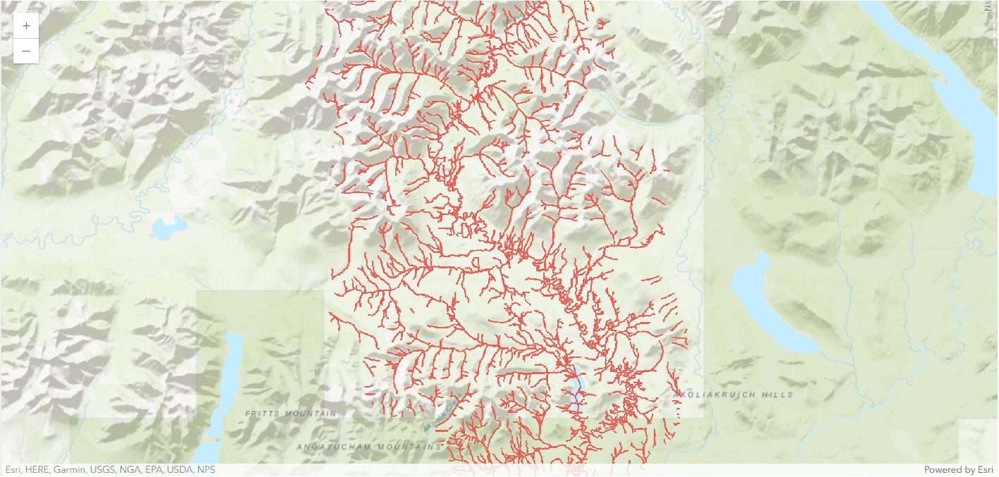
map1.zoom_to_layer(extracted_streams)Conclusion
The notebook presents the workflow showing how easily you can combine traditional morphological landform characteristics with deep learning methodologies using arcgis.learn to detect streams.