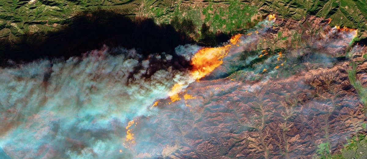
The Thomas Fire was a massive wildfire that started in early December 2017 in Ventura and Santa Barbara counties and grew into California's largest fire ever.
import arcgis
from arcgis import *
from arcgis.mapping import MapImageLayer
gis = GIS(profile="your_online_profile")Visualize the extent of damage
from ipywidgets import *

postfire = MapImageLayer('https://tiles.arcgis.com/tiles/DO4gTjwJVIJ7O9Ca/arcgis/rest/services/Digital_Globe_Imagery_Dec_11th/MapServer')

def side_by_side(address):
    location = geocode(address)[0]

    satmap1 = gis.map(location)
    satmap1.basemap = 'satellite'

    satmap2 = gis.map(location)
    satmap2.add_layer(postfire)

    satmap1.layout=Layout(flex='1 1', padding='6px', height='450px')
    satmap2.layout=Layout(flex='1 1', padding='6px', height='450px')

    box = HBox([satmap1, satmap2])
    return box
Nob Hill, Ventura, CA
side_by_side('Montclair Dr, Ventura, CA')
Vista Del Mar Hospital, Ventura, CA
side_by_side('801 Seneca St, Ventura, CA 93001')
Remote Sensing and Image Processing
landsat_item = gis.content.get('d9b466d6a9e647ce8d1dd5fe12eb434b')
landsat = landsat_item.layers[0]
landsat_item
Select before and after rasters
aoi = {'spatialReference': {'latestWkid': 3857, 'wkid': 102100}, 'type': 'extent',
       'xmax': -13305000, 'xmin': -13315000, 'ymax': 4106000, 'ymin': 4052000}

arcgis.env.analysis_extent = {"xmin":-13337766,"ymin":4061097,"xmax":-13224868,"ymax":4111469,
                              "spatialReference":{"wkid":102100,"latestWkid":3857}}

landsat.extent = aoi
import pandas as pd
from datetime import datetime
selected = landsat.filter_by(where="(Category = 1)",
time=[datetime(2017, 11, 15), datetime(2018, 1, 1)],
geometry=arcgis.geometry.filters.intersects(aoi))
df = selected.query(out_fields="AcquisitionDate, GroupName, CloudCover, DayOfYear",
order_by_fields="AcquisitionDate").sdf
df['AcquisitionDate'] = pd.to_datetime(df['AcquisitionDate'], unit='ms')
df.tail(5)| OBJECTID | AcquisitionDate | GroupName | CloudCover | DayOfYear | SHAPE | |
|---|---|---|---|---|---|---|
| 0 | 2083354 | 2017-11-23 18:34:42 | LC08_L1TP_042036_20171123_20200902_02_T1_MTL | 0.0444 | 36 | {"rings": [[[-13207893.09, 4198959.454999998],... |
| 1 | 2083355 | 2017-12-09 18:34:40 | LC08_L1TP_042036_20171209_20200902_02_T1_MTL | 0.2175 | 36 | {"rings": [[[-13208253.8058, 4199242.244499996... |
| 2 | 2083356 | 2017-12-25 18:34:42 | LC08_L1TP_042036_20171225_20200902_02_T1_MTL | 0.6571 | 36 | {"rings": [[[-13210387.2213, 4199063.157099999... |
prefire = landsat.filter_by('OBJECTID=' + str(df['OBJECTID'][0])) # 2017-11-23
midfire = landsat.filter_by('OBJECTID=' + str(df['OBJECTID'][1])) # 2017-12-09
Visual Assessment
from arcgis.raster.functions import *

apply(midfire, 'Natural Color with DRA')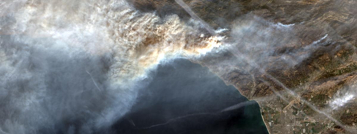
Visualize Burn Scars
Extract the [6, 4, 1] bands to improve visibility of fire and burn scars. This band combination pushes further into the SWIR range of the electromagnetic spectrum, where there is less susceptibility to smoke and haze generated by a burning fire.
extract_band(midfire, [6,4,1])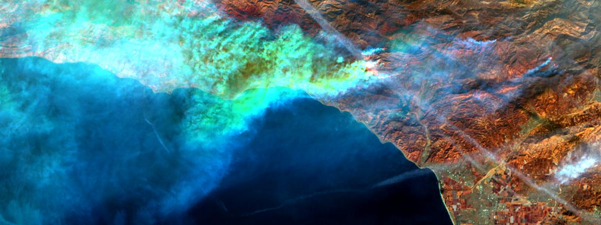
extract_band(prefire, [6,4,1])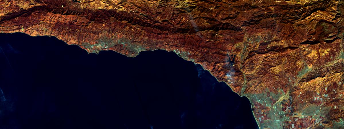
For comparison, the same area before the fire started shows no burn scar.
Quantitative Assessment
The Normalized Burn Ratio (NBR) can be used to delineate the burnt areas and identify the severity of the fire.
The formula for the NBR is very similar to that of NDVI except that it uses near-infrared band 5 and the short-wave infrared band 7:
\begin{align}
{\mathbf{NBR}} = \frac{\mathbf{B_5} - \mathbf{B_7}}{\mathbf{B_5} + \mathbf{B_7}} \
\end{align}
The NBR equation was designed to be calcualted from reflectance, but it can be calculated from radiance and digitalnumber(dn) with changes to the burn severity table below.
For a given area, NBR is calculated from an image just prior to the burn and a second NBR is calculated for an image immediately following the burn. Burn extent and severity is judged by taking the difference between these two index layers:
\begin{align}
{\Delta \mathbf{NBR}} = \mathbf{NBR{prefire}} - \mathbf{NBR{postfire}} \
\end{align}
The meaning of the ∆NBR values can vary by scene, and interpretation in specific instances should always be based on some field assessment. However, the following table from the USGS FireMon program can be useful as a first approximation for interpreting the NBR difference:
| \begin{align}{\Delta \mathbf{NBR}} \end{align} | Burn Severity |
|---|---|
| 0.1 to 0.27 | Low severity burn |
| 0.27 to 0.44 | Medium severity burn |
| 0.44 to 0.66 | Moderate severity burn |
| > 0.66 | High severity burn |
[Source: http://wiki.landscapetoolbox.org/doku.php/remote_sensing_methods:normalized_burn_ratio]
Use Band Arithmetic and Map Algebra
nbr_prefire  = band_arithmetic(prefire, "(b5 - b7) / (b5 + b7+1000)")
nbr_postfire = band_arithmetic(midfire, "(b5 - b7) / (b5 + b7+1000)")

nbr_diff = nbr_prefire - nbr_postfire
burnt_areas = colormap(remap(nbr_diff,
input_ranges=[0.1, 0.27, # low severity
0.27, 0.44, # medium severity
0.44, 0.66, # moderate severity
0.66, 1.00], # high severity burn
output_values=[1, 2, 3, 4],
no_data_ranges=[-1, 0.1], astype='u8'),
colormap=[[4, 0xFF, 0xC3, 0], [3, 0xFA, 0x8E, 0], [2, 0xF2, 0x55, 0], [1, 0xE6, 0, 0]])burnt_areas.draw_graph()<graphviz.graphs.Digraph at 0x22983c5bcd0>
Area calculation
ext = {"xmax": -13246079.10806628, "ymin": 4035733.9433013694, "xmin": -13438700.419344831, "ymax": 4158033.188557592,
       "spatialReference": {"wkid": 102100, "latestWkid": 3857}, "type": "extent"}
pixx = (ext['xmax'] - ext['xmin']) / 1200.0
pixy = (ext['ymax'] - ext['ymin']) / 450.0

res = burnt_areas.compute_histograms(ext, pixel_size={'x':pixx, 'y':pixy})

numpix = 0
histogram = res['histograms'][0]['counts'][1:]
for i in histogram:
    numpix += i
Report burnt area
from IPython.display import HTML
sqmarea = numpix * pixx * pixy # in sq. m
acres = 0.00024711 * sqmarea   # in acres

HTML('<h3>Thomas fire has consumed <i>{:,} acres</i>  till {}</h3>.'.format(int(acres), df.iloc[-1]['AcquisitionDate'].date()))
Thomas fire has consumed 307,428 acres till 2017-12-25
.import matplotlib.pyplot as plt
%matplotlib inline
plt.title('Distribution by severity', y=-0.1)
plt.pie(histogram, labels=['Low Severity', 'Medium Severity', 'Moderate Severity', 'High Severity']);
plt.axis('equal');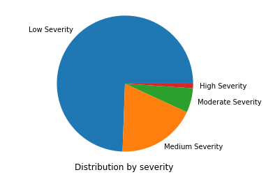
Visualize burnt areas
m = gis.map('Carpinteria, CA')
m
m.add_layer([midfire, burnt_areas])Raster to Feature layer conversion
Use Raster Analytics and Geoanalytics to convert the burnt area raster to a feature layer. The to_features() method converts the raster to a feature layer and create_buffers() fills holes in the features and dissolves them to output one feature that covers the extent of the Thomas Fire.
persisted_fire_output = burnt_areas.save()
persisted_fire_output_layer = persisted_fire_output.layers[0]
fire_item = persisted_fire_output_layer.to_features(output_name='ThomasFire_Boundary')

fire_layer = fire_item.layers[0]
fire_layer.filter = 'st_area_sh > 3000000'
fire = gis.content.search('ThomasFire_Boundary', 'Feature Layer')[0]
fire
Impact Assessment
Compute infrastructure and human impact
from arcgis.geoenrichment import enrich
from arcgis.features import SpatialDataFrame, FeatureLayer

sdf = pd.DataFrame.spatial.from_layer(fire.layers[0])

fire_geometry = sdf.iloc[0].SHAPE
sa_filter = geometry.filters.intersects(geometry=fire_geometry, sr=4326)

secondary_roads_layer = FeatureLayer("https://tigerweb.geo.census.gov/arcgis/rest/services/TIGERweb/Transportation_LargeScale/MapServer/1")
secondary_roads = secondary_roads_layer.query(geometry_filter=sa_filter, out_sr=4326)

local_roads_layer = FeatureLayer("https://tigerweb.geo.census.gov/arcgis/rest/services/TIGERweb/Transportation_LargeScale/MapServer/2")
local_roads = local_roads_layer.query(geometry_filter=sa_filter, out_sr=4326)

def age_pyramid(df):
    import warnings
    import seaborn as sns
    import matplotlib.pyplot as plt

    %matplotlib inline
    warnings.simplefilter(action='ignore', category=FutureWarning)
    pd.options.mode.chained_assignment = None
    plt.style.use('ggplot')

    df = df[[x for x in impacted_people.columns if 'MALE' in x or 'FEM' in x]]
    sf = pd.DataFrame(df.sum())
    sf['age'] = sf.index.str.extract('(\d+)').astype('int64')

    f = sf[sf.index.str.startswith('FEM')]
    m = sf[sf.index.str.startswith('MALE')]
    f = f.sort_values(by='age', ascending=False).set_index('age')
    m = m.sort_values(by='age', ascending=False).set_index('age')

    popdf = pd.concat([f, m], axis=1)
    popdf.columns = ['F', 'M']
    popdf['agelabel'] = popdf.index.map(str) + ' - ' + (popdf.index+4).map(str)
    popdf.M = -popdf.M

    sns.barplot(x="F", y="agelabel", color="#CC6699", label="Female", data=popdf, edgecolor='none')
    sns.barplot(x="M",  y="agelabel", color="#008AB8", label="Male",   data=popdf,  edgecolor='none')
    plt.ylabel('Age group')
    plt.xlabel('Number of people');
    return plt;
Visualize affected roads on map
impactmap = gis.map('Carpinteria, CA')
impactmap.basemap = 'streets'

impactmap
impactmap.draw([local_roads, secondary_roads])Age Pyramid of affected population
impacted_people = enrich(sdf, 'Age')
age_pyramid(impacted_people);