Introduction
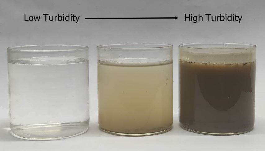
Turbidity represents the level of suspended sediments in water also indicating water clarity or how clear is the water. It is mainly caused by the presence of silt, algae in a water body, or industrial waste disposed in the rivers by mining activity, industrial operations, logging, etc.
Traditionally, turbidity is analyzed by evaluating water samples taken during field measurements. However, field studies are expensive, time and labor intensive, besides, during lockdown field surveys cannot be undertaken. Thus, a good alternative to field survey measurements is satellite remote sensing data, which can capture both spatial and temporal variations in river turbidity levels. Accordingly, Sentinel-2 multispectral data is used in the current study to evaluate the changes in river turbidity during COVID-19 lockdown, near the holy city of Allahabad, India.
Allahabad, situated in the northern part of India, is at the confluence of two major rivers: Ganga and its tributary river Yamuna. The point of confluence is a sacred place for Hindus where thousands of devotees gather everyday by the banks of the river to offer prayers. Millions of people depend on the waters from these rivers yet both rivers are heavily polluted by industrial waste, by sewage and even by the remains of the many bodies cremated on their banks. On March 25, 2020, India announced a lockdown for controlling the spread of COVID-19 leading to complete shutdown of industries and restricted human movement. The lockdown resulted in reduction of turbidity thereby improving water quality in rivers throughout the country. This notebook will elaborate the steps to measure this change in turbidity using ArcGIS API for Python.
Necessary Imports
import pandas as pd
from ipywidgets import HBox, VBox, Label, Layout


import arcgis
from arcgis.features import GeoAccessor, GeoSeriesAccessor
from arcgis.raster.analytics import convert_feature_to_raster, convert_raster_to_feature
from arcgis.raster.functions import extract_band, greater_than, clip, remap, colormap, stretch
from arcgis.features.analysis import dissolve_boundaries
Connect to your GIS
from arcgis import GIS
agol_gis = GIS(profile='your_online_profile')
ent_gis = GIS(profile='your_enterprise_profile')
Get the data for analysis
Sentinel-2 Views is used in the analysis, this multitemporal layer consists 13 bands with 10, 20, and 60m spatial resolution. The imagery layer is rendered on-the-fly and available for visualization and analytics. This imagery layer pulls directly from the Sentinel-2 on AWS collection and is updated daily with new imagery.
s2 = agol_gis.content.get('fd61b9e0c69c4e14bebd50a9a968348c')
sentinel = s2.layers[0]
s2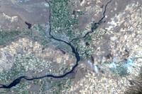
A feature layer was published which represents the extent of study area. This feature will be used for extracting Sentinel-2 tiles of study area.
aoi1 = agol_gis.content.search('title:allahabad_aoi owner:api_data_owner', 'Feature Layer Collection')[0]
aoi1
Methodology
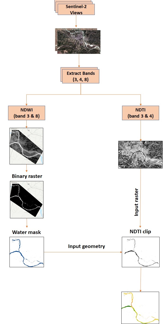
The above diagram encapsulates the overall methodology that has been followed in the estimation of the river turbidity.
Prepare data for analysis
Sentinel-2 Views imagery layer consists data for the whole world and span different time periods. Thus, the first step is to filter out the data for the rivers in Allahabad region prior to and during the lockdown period.
Create geometry of area of interest (AOI)
The geometry of AOI is created for filtering out the Sentinel-2 tiles for the study area.
aoi_layer = aoi1.layers[0]
aoi_feature = aoi_layer.query(where='fid=1')
aoi_geom = aoi_feature.features[0].geometry
aoi_geom['spatialReference'] = {'wkid':3857}
Filter out sentinel-2 tiles
m = agol_gis.map('Allahabad, India')
m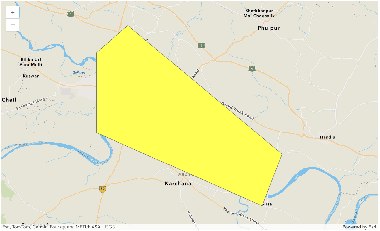
m.content.add(
    item=aoi1
)m.zoom_to_layer(aoi1)Before lockdown
Sentinel-2 tiles were filtered out for before lockdown scenario using query function on the basis of AcquistionDate column. Category represents source of data, for the current analysis Category=1 was used which means Sentinel-2 Level-1 data. Sentinel-2 tiles were filtered out for the before lockdown scenario from March 9, 2020 to March 11, 2020.
from datetime import datetime
selected = sentinel.filter_by(where="(Category = 1)",
                             time=[datetime(2020, 3, 9), datetime(2020, 3, 11)],
                             geometry=arcgis.geometry.filters.intersects(aoi_geom))
df = selected.query(out_fields="AcquisitionDate, GroupName, CloudCover, DayOfYear",
                   order_by_fields="AcquisitionDate").sdf

df['AcquisitionDate'] = pd.to_datetime(df['acquisitiondate'], unit='ms')
df| objectid | acquisitiondate | groupname | cloudcover | dayofyear | shape_Length | shape_Area | SHAPE | AcquisitionDate | |
|---|---|---|---|---|---|---|---|---|---|
| 0 | 10003774 | 2020-03-09 05:21:34 | 20200309T052134_44RPP_0 | 0 | 69 | 411289.670549 | 1.001614e+10 | {"rings": [[[9225034.6736, 3024534.521499999],... | 2020-03-09 05:21:34 |
| 1 | 10003775 | 2020-03-09 05:21:38 | 20200309T052137_44RNP_0 | 0 | 69 | 486307.001820 | 1.478067e+10 | {"rings": [[[9138906.555100001, 3025524.7907],... | 2020-03-09 05:21:38 |
| 2 | 10003776 | 2020-03-09 05:21:49 | 20200309T052148_44RPN_0 | 0 | 69 | 357605.263126 | 6.801910e+09 | {"rings": [[[9198149.502, 2913289.101599999], ... | 2020-03-09 05:21:49 |
| 3 | 10003777 | 2020-03-09 05:21:52 | 20200309T052152_44RNN_0 | 0 | 69 | 482722.878472 | 1.456361e+10 | {"rings": [[[9137984.507800002, 2913901.974500... | 2020-03-09 05:21:52 |
Sentinel-2 tile of OBJECTID=10003775 was selected which represents before lockdown turbidity conditions.
tile1 = sentinel.filter_by('OBJECTID=10003775')
tile1.extent = m.extent
tile1.save('s2_allbd_20200309', gis=ent_gis)
tile1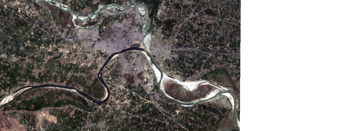
During lockdown
Sentinel-2 tiles were filtered out for during lockdown scenario using query function on the basis of AcquistionDate column. Sentinel-2 tiles were filtered out for the before lockdown scenario from April 9, 2020 to April 14, 2020.
from datetime import datetime
selected = sentinel.filter_by(where="(Category = 1)",
                             time=[datetime(2020, 4, 9), datetime(2020, 4, 14)],
                             geometry=arcgis.geometry.filters.intersects(aoi_geom))
df = selected.query(out_fields="AcquisitionDate, GroupName, CloudCover, DayOfYear",
                   order_by_fields="AcquisitionDate").sdf

df['AcquisitionDate'] = pd.to_datetime(df['acquisitiondate'], unit='ms')
df| objectid | acquisitiondate | groupname | cloudcover | dayofyear | shape_Length | shape_Area | SHAPE | AcquisitionDate | |
|---|---|---|---|---|---|---|---|---|---|
| 0 | 10304744 | 2020-04-13 05:21:34 | 20200413T052134_44RPP_0 | 0.0207 | 104 | 411250.271731 | 1.001344e+10 | {"rings": [[[9225023.4659, 3024534.6838000007]... | 2020-04-13 05:21:34 |
| 1 | 10481214 | 2020-04-13 05:21:38 | 20200413T052137_44RNP_0 | 0.0004 | 104 | 486307.001820 | 1.478067e+10 | {"rings": [[[9138906.555100001, 3025524.7907],... | 2020-04-13 05:21:38 |
| 2 | 10415547 | 2020-04-13 05:21:49 | 20200413T052148_44RPN_0 | 0.0000 | 104 | 357554.873540 | 6.799904e+09 | {"rings": [[[9198094.4782, 2913289.7751], [916... | 2020-04-13 05:21:49 |
| 3 | 10415548 | 2020-04-13 05:21:52 | 20200413T052152_44RNN_0 | 0.0000 | 104 | 482722.878472 | 1.456361e+10 | {"rings": [[[9137984.507800002, 2913901.974500... | 2020-04-13 05:21:52 |
Sentinel-2 tile of OBJECTID=10481214 was selected which represents during lockdown turbidity conditions.
tile2 = sentinel.filter_by('OBJECTID=10481214')
tile2.extent = m.extent
tile2.save('s2_allbd_20200413', gis=ent_gis)
tile2
tiles = ent_gis.content.search('title:s2_allbd_')
tilestimestamps=set([layer.title[-8:] for layer in tiles])
timestamps=[t.strftime('%Y%m%d') for t in sorted([datetime.strptime(t,'%Y%m%d') for t in timestamps])]Generate water body mask
Extract bands
Green (band 3), Red (band 4) and NIR (band 8) bands were extracted from the Sentinel-2 tiles for NDWI and NDTI calculation.
def extract_green_band(tiles):
    print('extracting green band',end='\r')
    green_band = extract_band(tiles, [3])
    return green_band
def extract_red_band(tiles):
print('extracting red band',end='\r')
red_band = extract_band(tiles, [4])
return red_banddef extract_nir_band(tiles):
print('extracting nir band',end='\r')
nir_band = extract_band(tiles, [8])
return nir_bandCreate normalized difference water (NDWI) index raster
Normalized difference water index (NDWI) is a satellite based index used for mapping and detecting the surface water bodies. Water absorbs electromagnetic radiation in visible to infrared spectrum, that is why Green and Near Infrared bands are used to detect the water bodies. In the current study, band 3 (green) and band 8 (NIR) of Sentinel-2 are used for generating NDWI raster. Here, t represents timestamps.
def create_ndwi_raster(green_band, nir_band, t, aoi_geom):
    print('creating ndwi raster',end='\r')
    ndwi = (green_band - nir_band)/(green_band + nir_band)
    c_ndwi = clip(ndwi, aoi_geom)
    ndwi_s = c_ndwi.save("ndwi_allbdt"+t, gis=ent_gis)
    ndwi_lyr = ndwi_s.layers[0]
    return ndwi_lyr
Create binary raster
Binary raster is created from NDWI raster using a threshold value. The binary raster consists of two classes of water and non-water pixels where pixels with value greater than 0.03 are considered as water. Accordingly, this threshold value of 0.03 is used for creating the binary raster using the greater_than function. Here, t represents timestamps.
def create_binary_raster(ndwi_lyr, t):
    print('creating binary raster',end='\r')
    binary_raster = greater_than([ndwi_lyr, 0.03],
                              extent_type='FirstOf',
                              cellsize_type='FirstOf',
                              astype='U16')
    binary_ras = binary_raster.save("binaryrast_"+t, gis=ent_gis)
    binaryras_lyr = binary_ras.layers[0]
    return binaryras_lyr
Create water body mask
Convert binary raster to feature layer
The binary rasters are converted to feature layer for extracting the boundaries of the water bodies. Here, t represents timestamps.
def create_binary_poly(binaryras_lyr, t):
    print('creating binary feature layer',end='\r')
    binary_poly = convert_raster_to_feature(binaryras_lyr,
                                          field='Value',
                                          output_type='Polygon',
                                          simplify=True,
                                          output_name='binary_poly'+t,
                                          gis=ent_gis)
    return binary_poly
Extract water polygons
In the feature layer returned above, 'gridcode=0' represents non water class and 'gridcode=1' represents water class. Thus, the water polygons with 'gridcode=1 are selected using the query function from the dataframe of the feature layer and saved into a new feature layer created using gis.content.import function consisting of these water polygons. Here, t represents timestamps.
def extract_water_polygons(binary_poly, t):
    print('extracting water polygon',end='\r')
    dfm=binary_poly.layers[0].query('gridcode=1').sdf
    water_poly=gis_ent.content.import_data(dfm, title='wpoly'+t)
    return water_poly
The features of water_poly were dissolved using dissolve_boundaries function. The features were dissolved on the basis of gridcode column.
Finally the features in the layer water_poly are dissolved using dissolve_boundaries function on the basis of gridcode column to obtain the water body mask in the following.
def dissolve_water_features(water_poly, t):
    print('dissolving water features',end='\r')
    diss_f = dissolve_boundaries(water_poly,
                                 dissolve_fields=['gridcode'],
                                 output_name='dissolve_poly'+t,
                                 gis=ent_gis,
                                 multi_part_features=True)
    return diss_f
Normalized difference turbidity index
The Normalize Difference Turbidity Index (NDTI) which is estimated using the spectral reflectance values of the water pixels is used to estimate the turbidity in water bodies. It uses the phenomenon that the electromagnetic reflectance is higher in green spectrum than the red spectrum for clear water. Hence, with increase in turbidity the reflectance of red spectrum also increases. Accordingly, in the current study, Sentinel-2 green (band 3) and red (band 4) bands are used to create the NDTI raster in the following. Here, t represents timestamps.
def create_ndti_ras(red_band, green_band, t):
    print('creating ndti raster',end='\r')
    ndti = (red_band - green_band)/(red_band + green_band)
    ndti_s = ndti.save("ndti_allbd"+t, gis=ent_gis)
    ndti_lyr = ndti_s.layers[0]
    return ndti_lyr
Turbidity raster for water bodies
Once the NDTI raster is prepared, its portion for the water body is extracted using the water body mask obtained earlier. To do so, fwe start by creating the geometry of dissolve_f as follows:
def create_water_geom(diss_f):
    print('creating geometry',end='\r')
    aoi2_layer = diss_f.layers[0]
    aoi2_feature = aoi2_layer.query(where='gridcode=1')
    aoi2_geom = aoi2_feature.features[0].geometry
    aoi2_geom['spatialReference'] = {'wkid':3857}
    return aoi2_geom
Second step is to clip the NDTI rasters with the geometry of dissolve_f raster. Here, t represents timestamps.
def clip_water_ndti_ras(ndti_lyr, aoi2_geom, t):
    print('clipping ndti raster with water boundary',end='\r')
    clip_ndti = clip(ndti_lyr, aoi2_geom)
    clip_ndti_ras = clip_ndti.save("cl_ndti"+t, gis=ent_gis)
    return clip_ndti_ras
Third step is to apply colormap for visualizing the results. Here, t represents timestamps.
def stretch_ndti_ras(clip_ndti_ras, t):
    print('clipping stretch ndti raster',end='\r')
    stretch_rs = colormap(stretch(clip_ndti_ras.layers[0],
                                  stretch_type='PercentClip',
                                  min=0,
                                  max=255),
                          colormap_name="Condition Number")
    ndti_cmap = stretch_rs.save("ndti_cmapr"+t, gis=ent_gis)
    return stretch_ras
Finally, all of the above mentioned functions are used inside a loop and applied on the satellite imagery of the river from two different time periods: one before lockdown (March 9, 2020) and the second, during the lockdown period (April 13, 2020), to visualize and compare the difference in the turbidity levels.
for t in timestamps:

    print(f'Processing layers for :{t}\n')
    tiles = ent_gis.content.search(f's2_allbd_{t}')[0].layers[0]
    green_band=extract_green_band(tiles=tiles)
    red_band=extract_red_band(tiles=tiles)
    nir_band=extract_nir_band(tiles=tiles)
    ndwi_lyr=create_ndwi_raster(green_band=green_band, nir_band=nir_band, t=t, aoi_geom=aoi_geom)
    binaryras_lyr=create_binary_raster(ndwi_lyr=ndwi_lyr, t=t)
    binary_poly=create_binary_poly(binaryras_lyr=binaryras_lyr, t=t)
    water_poly=extract_water_polygons(binary_poly=binary_poly, t=t)
    diss_f=dissolve_water_features(water_poly=water_poly, t=t)
    ndti_lyr=create_ndti_ras(green_band=green_band, red_band=red_band, t=t)
    aoi2_geom=create_water_geom(diss_f=diss_f)
    clip_ndti_ras=clip_water_ndti_ras(ndti_lyr=ndti_lyr, aoi2_geom=aoi2_geom, t=t)
    stretch_ras=stretch_ndti_ras(clip_ndti_ras=clip_ndti_ras, t=t)
    print(f'Processing completed for :{t}\n')
Processing layers for :20200309 Processing completed for :20200309 Processing layers for :20200413 Processing completed for :20200413
Visualize results
Result Visualization
The NDTI rasters and their corresponding Sentinel-2 tiles are now accessed from the portal and used for visualization.
ras1 = ent_gis.content.search('ndti_cmap20200309', 'Imagery Layer')[0]
ras2 = ent_gis.content.search('ndti_cmap20200413', 'Imagery Layer')[0]
ras3 = ent_gis.content.search('s2_allbd_20200309', 'Imagery Layer')[0]
ras4 = ent_gis.content.search('s2_allbd_20200413', 'Imagery Layer')[0]
Create map widgets
4 map wigets are created representing the NDTI raster and corresponding Sentinel-2 for 9th March (before lockdown) and 13th April (during lockdown).
map1 = ent_gis.map("Allahabad, India")
map1.basemap.basemap = 'terrain'
map1.content.add(ras1)
map2 = ent_gis.map("Allahabad, India")
map2.basemap.basemap = 'terrain'
map2.content.add(ras2)
map3 = ent_gis.map("Allahabad, India")
map3.content.add(ras3)
map4 = ent_gis.map("Allahabad, India")
map4.content.add(ras4)
Synchronize web maps
All the maps are synchronized with each other using MapView.sync_navigation functionality. It helps in comparing the river turbidity before and during lockdown. Detailed description about advanced map widget options can be referred here
map1.sync_navigation(map2)
map2.sync_navigation(map3)
map3.sync_navigation(map4)
Set the map layout
Hbox and Vbox were used to set the layout of map widgets.
hbox_layout = Layout()
hbox_layout.justify_content = 'space-around'

hb1,hb2=HBox([Label('NDTI (March 9, 2020)'),Label('NDTI (April 13, 2020)')]),\
                HBox([Label('Sentinel-2 (March 9, 2020)'),Label('Sentinel-2 (April 13, 2020)')])
hb1.layout,hb2.layout=hbox_layout,hbox_layout
Interpretation of results
VBox([hb1,HBox([map1,map2]),hb2, HBox([map3,map4])])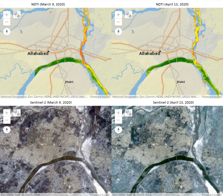
The maps above show the spatio-temporal variation in turbidity of the Ganga and Yamuna rivers due to Covid-19 lockdown. The satellite imageries used in the analysis are from before lockdown, dated March 9, 2020 (bottom-left), and during the lockdown, dated April 13, 2020 (botton-right).
It can be seen that turbidity declined in both the Ganga and Yamuna rivers during lockdown as indicated by the Red pixels representing high turbidity, turning to Orange, Yellow and finally Green, which is the lowest level of turbidity. Compared to Yamuna, the Ganga river had a significant impact on turbidity due to lockdown. The complete stretch of Ganga turned from red and yellow to mostly green pixels. The turbidity at the confluence point also declined followed by a decline in the stretch downstream.
Conclusion
Ganga and Yamuna rivers are among the world's most polluted due to dumping of waste from industrial and religious activities as indicated by their highly turbid water. During the lockdown period, pollution levels fell dramatically in both rivers due to complete shutdown of the above-mentioned functions. This change was investigated using Sentinel-2 satellite imageries of the river stretches, before and during the lockdown periods, with results suggesting substantial decrease in turbidity levels thereby validating the same. The same methodology can be implemented to study the changes in river turbidity for other regions with Sentinel-2 data using ArcGIS platform.
Literature resources
| Literature | Source | Link |
|---|---|---|
| Research Paper | Changes in turbidity along Ganga River using Sentinel-2 satellite data during lockdown associated with COVID-19 | https://www.tandfonline.com/doi/full/10.1080/19475705.2020.1782482 |
| Research Paper | Water Turbidity Assessment in Part of Gomti River Using High Resolution Google Earth Quickbird satellite data | https://geospatialworldforum.org/2011/proceeding/pdf/Shivangifullpaper.pdf |