This sample shows how the network module of the ArcGIS API for Python can be used to construct service areas. In this sample, we generate service areas for two of the fire stations in central Tokyo, Japan. We later observe how the service area varies by time of day for a fire station in the city of Los Angeles.
Service areas
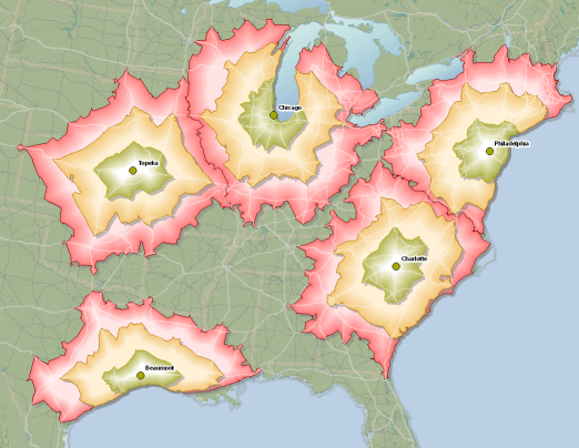
A network service area is a region that encompasses all accessible streets (that is, streets that are within a specified impedance). For instance, the 5-minute service area for a point on a network includes all the streets that can be reached within five minutes from that point.
Service areas also help evaluate accessibility. Concentric service areas show how accessibility varies. Once service areas are created, you can use them to identify how much land, how many people, or how much of anything else is within the neighborhood or region.
Service area solver provides functionality for finding out how far a vehicle could go within a specified time or distance limit.
Connect to the GIS
Establish a connection to your organization which could be an ArcGIS Online organization or an ArcGIS Enterprise. To be able to run the code in this sample notebook, you would need to provide credentials of a user within an ArcGIS Online organization.
from datetime import datetime
from arcgis.gis import GIS
from arcgis.map.symbols import PictureMarkerSymbolEsriPMS, SimpleFillSymbolEsriSFS
from arcgis.map.popups import PopupInfo

my_gis = GIS(profile='your_online_profile')
Create a Network Layer
To perform any network analysis (such as finding the closest facility, the best route between multiple stops, or service area around a facility), you would need to create a NetworkLayer object. In this sample, since we are creating service areas, we need to create a ServiceAreaLayer which is a type of NetworkLayer.
To create any NetworkLayer object, you would need to provide the URL to the appropriate network analysis service. Hence, in this sample, we provide a serviceArea URL to create a ServiceAreaLayer object.
Since all ArcGIS Online organizations already have access to those routing services, you can access this URL through the GIS object's helperServices property. If you have your own ArcGIS Server based map service with network analysis capability enabled, you would need to provide the URL for this service.
Let us start by importing the network module
import arcgis.network as networkservice_area_url = my_gis.properties.helperServices.serviceArea.url
service_area_url'https://route.arcgis.com/arcgis/rest/services/World/ServiceAreas/NAServer/ServiceArea_World'
sa_layer = network.ServiceAreaLayer(service_area_url, gis=my_gis)Create fire station facility layer
We obtained the coordinates of two fire stations in Tokyo. We construct Feature and FeatureSet objects to represent them.
fire_station_1_coord = '139.546910,35.695729'
fire_station_2_coord = '139.673726,35.697988'

from arcgis.features import Feature, FeatureSet

f1 = Feature(geometry={'x':float(fire_station_1_coord.split(',')[0]),
                      'y':float(fire_station_1_coord.split(',')[1])})

f2 = Feature(geometry={'x':float(fire_station_2_coord.split(',')[0]),
                      'y':float(fire_station_2_coord.split(',')[1])})

fire_station_fset = FeatureSet([f1,f2], geometry_type='esriGeometryPoint',
                            spatial_reference={'latestWkid': 4326})
Let us display the fire stations on a map
map1 = my_gis.map('Tokyo')
map1
fire_truck_symbol = PictureMarkerSymbolEsriPMS(**{"type":"esriPMS",
                     "url":"http://static.arcgis.com/images/Symbols/SafetyHealth/FireTruck.png",
                     "contentType": "image/png", "width":20, "height":20})

map1.content.draw(fire_station_fset, symbol=fire_truck_symbol)
Compute the service area
To compute the service area (area accessible to each facility based on drive times), we use the solve_service_area() method of a ServiceAreaLayer object. As the fire trucks will be travelling away from the stations, we need to specify the direction of travel in the travel_direction parameter. Also, since for the type of vehicles is fire trucks, we could specify the travel mode to make it easier to supply all other related parameters.
travel_modes = sa_layer.retrieve_travel_modes()
truck_mode = [t for t in travel_modes['supportedTravelModes'] if t['name'] == 'Trucking Time'][0]

result = sa_layer.solve_service_area(fire_station_fset, default_breaks=[5,10,15],
                                     travel_direction='esriNATravelDirectionFromFacility',
                                     travel_mode=truck_mode)
Read the result back as a FeatureSet
The result variable contains the service area as a dictionary. We inspect its keys and construct Feature and FeatureSet objects out of it to display in the map
result.keys()dict_keys(['messages', 'saPolygons'])
result['saPolygons'].keys()dict_keys(['geometryType', 'fieldAliases', 'spatialReference', 'features'])
poly_feat_list = []
for polygon_dict in result['saPolygons']['features']:
    f1 = Feature(polygon_dict['geometry'], polygon_dict['attributes'])
    poly_feat_list.append(f1)
service_area_fset = FeatureSet(poly_feat_list,
geometry_type=result['saPolygons']['geometryType'],
spatial_reference= result['saPolygons']['spatialReference'])Let us inspect the service area as a Pandas DataFrame to understand the attribute information
service_area_fset.sdf| FacilityID | FromBreak | Name | ObjectID | Shape_Area | Shape_Length | ToBreak | SHAPE | |
|---|---|---|---|---|---|---|---|---|
| 0 | 1 | 10 | Location 1 : 10 - 15 | 1 | 0.002705 | 0.779069 | 15 | {'rings': [[[139.5388164520001, 35.71464347800... |
| 1 | 1 | 5 | Location 1 : 5 - 10 | 2 | 0.001400 | 0.393997 | 10 | {'rings': [[[139.55925560000003, 35.7247486110... |
| 2 | 1 | 0 | Location 1 : 0 - 5 | 3 | 0.000453 | 0.109327 | 5 | {'rings': [[[139.55229377700005, 35.7074565890... |
| 3 | 2 | 10 | Location 2 : 10 - 15 | 4 | 0.003424 | 1.058613 | 15 | {'rings': [[[139.705453873, 35.764051437000035... |
| 4 | 2 | 5 | Location 2 : 5 - 10 | 5 | 0.001749 | 0.429482 | 10 | {'rings': [[[139.68995857200002, 35.7177867890... |
| 5 | 2 | 0 | Location 2 : 0 - 5 | 6 | 0.000554 | 0.121896 | 5 | {'rings': [[[139.67423820500005, 35.7097034450... |
Visualize the service area on the map
From the DataFrame above, we know, there are 3 service area polygons for each fire station. The drive times are given as a range between FromBreak and ToBreak columns. Let us use this information to visualize the polygons with different colors and appropriate popup messags on the map
colors = {5: [0, 128, 0, 90],
10: [255, 255, 0, 90],
15: [255, 0, 0, 90]}
fill_symbol = SimpleFillSymbolEsriSFS(**{"type": "esriSFS","style": "esriSFSSolid",
"color": [115,76,0,255]})for service_area in service_area_fset.features:
#set color based on drive time
fill_symbol.color = colors[service_area.attributes['ToBreak']]
#set popup
popup=PopupInfo(**{"title": "Service area",
"description": "{} minutes".format(service_area.attributes['ToBreak'])})
map1.content.draw(service_area.geometry, symbol=fill_symbol, popup=popup)Click the drive time areas to explore their attributes. Because the content of the pop-ups may include HTML source code, it is also possible to have the pop-up windows include other resources such as tables and images.
Constructing service areas for different times of the day
The service areas for the facilities may look different depending on what time of day a vehicle would start driving. Therefore, we will run the solver using multiple day times for the time_of_day parameter to be able to compare visually the difference between the service areas. We will generate service areas for the following times: 6am, 10am, 2pm, 6pm, and 10pm.
In the following example, we assume that the facility is in the downtown of Los Angeles and we want to generate drive time areas at different times during the same day.
times = [datetime(2017, 6, 10, h).timestamp() * 1000
for h in [6, 10, 14, 18, 22]]
# fire station location
fire_station = '-118.245847, 34.038608'
#loop through each time of the day and compute the service area
sa_results = []
for daytime in times:
result = sa_layer.solve_service_area(facilities=fire_station, default_breaks=[5,10,15],
travel_direction='esriNATravelDirectionFromFacility',
time_of_day=daytime, time_of_day_is_utc=False)
sa_results.append(result)The service area has been computed, we process it to generate a list of FeatureSet objects to animate on the map
LA_fset_list=[]
for result in sa_results:
poly_feat_list = []
for polygon_dict in result['saPolygons']['features']:
f1 = Feature(polygon_dict['geometry'], polygon_dict['attributes'])
poly_feat_list.append(f1)
service_area_fset = FeatureSet(poly_feat_list,
                         geometry_type=result['saPolygons']['geometryType'],
                         spatial_reference= result['saPolygons']['spatialReference'])
LA_fset_list.append(service_area_fset)Draw and animate the results on a map
map2= my_gis.map("Los Angeles, CA")
map2
import time
map2.content.remove_all()

times = ['6 am', '10 am', '2 pm', '6 pm', '10 pm']
j=0
time.sleep(5)

for fset in LA_fset_list:
    print(times[j])
    map2.content.draw(fset)
    j+=1
    time.sleep(1)
6 am 10 am 2 pm 6 pm 10 pm
Thus from the animation above, we notice the service area is smallest at 6 AM and increases progressively later during the day.