- 🔬 Data Science
- 🖥️ Requires RasterAnalytics Portal Configuration
- 🖥️ Requires GeoEnrichment Portal Configuration
- 🖥️ Requires GeoAnalytics Portal Configuration
The Pawnee Fire was a large wildfire that burned in Lake County, California. The fire started on June 23, 2018 and burned a total of 15,185 acres (61 km2) before it was fully contained on July 8, 2018.

Remote Sensing using Sentinel-2 data
from datetime import datetime
import warnings

from IPython.display import HTML
import pandas as pd
import matplotlib.pyplot as plt
import seaborn as sns

import arcgis
from arcgis import GIS
from arcgis.raster.functions import *
from arcgis.geoanalytics.use_proximity import create_buffers
from arcgis.geoenrichment import enrich
from arcgis.features import SpatialDataFrame
from arcgis.raster.analytics import create_image_collection
from arcgis.raster.analytics import list_datastore_content

gis= GIS('https://pythonapi.playground.esri.com/portal', 'arcgis_python', 'amazing_arcgis_123')
Data Preparation
In this analysis, we will be using Sentinel-2 data.
Sentinel-2 is an Earth observation mission developed by ESA as part of the Copernicus Programme to perform terrestrial observations in support of services such as forest monitoring, land cover change detection, and natural disaster management.
In this analysis data downloaded from https://earthexplorer.usgs.gov/ is used for creating hosted image service. We add the data to the datastore and we then run the create_image_collection function which creates a collection with the input_rasters specified and publishes the collection as an image service.
We use list_datasore_content() in order to see the contents in the rasterstore.
list_datastore_content("/rasterStores/LocalRasterStore")['/rasterStores/LocalRasterStore/Hosted_GeneratedRasterProduct_AANS52.crf/', '/rasterStores/LocalRasterStore/L1C_T10SEJ_A015697_20180624T190108.zip', '/rasterStores/LocalRasterStore/me.txt', '/rasterStores/LocalRasterStore/m_7013bfcd7273e0a4a779fce061167d5c/', '/rasterStores/LocalRasterStore/m_b5f745ad6ef601d5e6adf104c8b4ef70/', '/rasterStores/LocalRasterStore/m_d0221b176ab5ed2398828b8079d62ef8/', '/rasterStores/LocalRasterStore/pawnee_fire_multispectral/', '/rasterStores/LocalRasterStore/pool_chips_1/', '/rasterStores/LocalRasterStore/pool_chips_2/', '/rasterStores/LocalRasterStore/S2A_MSIL1C_20180624T184921_N0206_R113_T10SEJ_20180624T234856.SAFE/', '/rasterStores/LocalRasterStore/S2B_MSIL1C_20180622T185919_N0206_R013_T10SEJ_20180622T205930.SAFE/', '/rasterStores/LocalRasterStore/sentinel_data/']
sentinel_collection = create_image_collection(image_collection="pawnee_fire_multispectral",
                      input_rasters=["/rasterStores/LocalRasterStore/S2A_MSIL1C_20180624T184921_N0206_R113_T10SEJ_20180624T234856.SAFE",
                                     "/rasterStores/LocalRasterStore/S2B_MSIL1C_20180622T185919_N0206_R013_T10SEJ_20180622T205930.SAFE"],
                      raster_type_name="Sentinel-2",
                      raster_type_params={"productType":"All","processingTemplate":"Multispectral"},
                      context={"image_collection_properties":{"imageCollectionType":"Satellite"},"byref":True}, gis = gis)
sentinel = sentinel_collection.layers[0]Select before and after rasters
aoi = {'spatialReference': {'latestWkid': 3857, 'wkid': 102100},
 'xmax': -13643017.100720055,
 'xmin': -13652113.10708598,
 'ymax': 4739654.477447927,
 'ymin': 4731284.622850712}
arcgis.env.analysis_extent = aoi
sentinel.extent = aoi
selected = sentinel.filter_by(where="acquisitiondate BETWEEN timestamp '2018-06-15 00:00:00' AND timestamp '2018-06-24 19:59:59'",
geometry=arcgis.geometry.filters.intersects(aoi))
df = selected.query(out_fields="*", order_by_fields="OBJECTID ASC").df
df['AcquisitionDate'] = pd.to_datetime(df['AcquisitionDate'], unit='ms')
df.tail(40)| AcquisitionDate | Category | CenterX | CenterY | CloudCover | CreationTime | Creator | GroupName | HighPS | LowPS | ... | SOrder | SensingOrbit | SensorName | Shape_Area | Shape_Length | StereoID | Tag | Thumbnail | ZOrder | SHAPE | |
|---|---|---|---|---|---|---|---|---|---|---|---|---|---|---|---|---|---|---|---|---|---|
| 0 | 2018-06-24 18:49:21.024 | 1 | -1.362127e+07 | 4.758219e+06 | 0 | 1548778472000 | rjackson | MTD_MSIL1C | 60 | 60 | ... | None | 113 | Sentinel-2A | 2.008228e+10 | 562920.108277 | None | MS | None | None | {'rings': [[[-13549665.930399999, 4828694.125]... |
| 1 | 2018-06-22 18:59:19.024 | 1 | -1.364188e+07 | 4.762904e+06 | 0 | 1548778472000 | rjackson | MTD_MSIL1C | 60 | 60 | ... | None | 13 | Sentinel-2B | 1.417943e+10 | 488606.729731 | None | MS | None | None | {'rings': [[[-13611168.835900001, 4689604.0966... |
2 rows × 26 columns
prefire = sentinel.filter_by('OBJECTID=2')
midfire = sentinel.filter_by('OBJECTID=1')
Visual Assessment
truecolor = extract_band(midfire, [4,3,2])
truecolor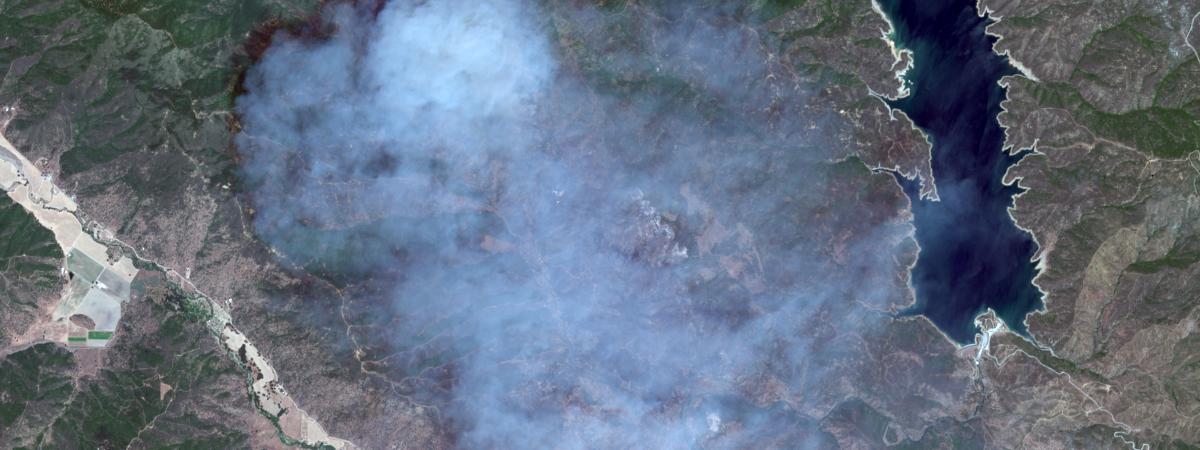
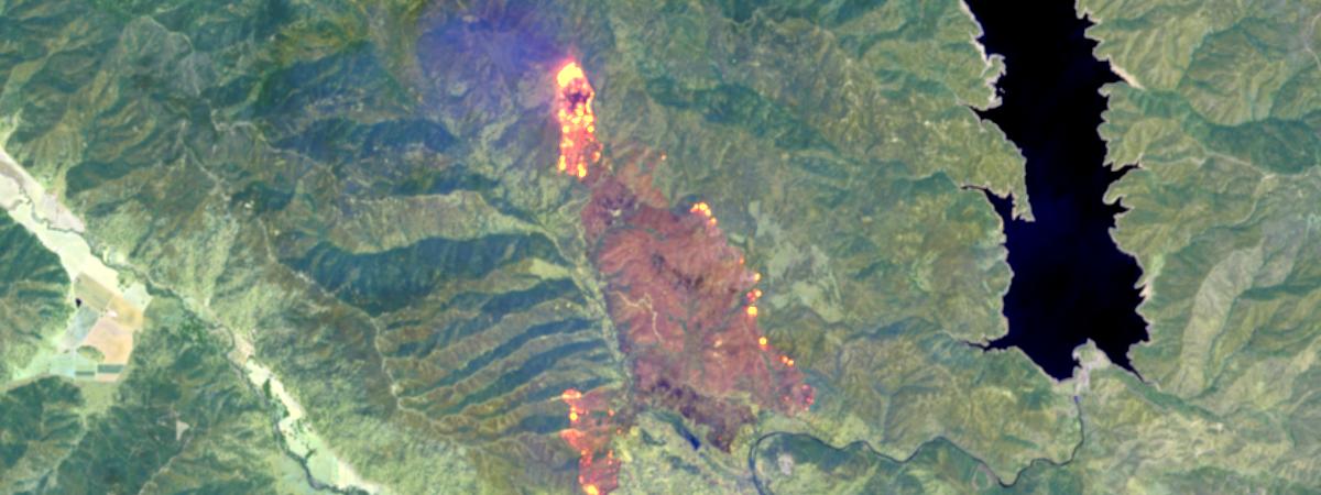
Visualize Burn Scars
We extract the [13, 12, 4] bands to improve visibility of fire and burn scars. This band combination pushes further into the SWIR range of the electromagnetic spectrum, where there is less susceptibility to smoke and haze generated by a burning fire.
extract_band(midfire, [13,12,4])
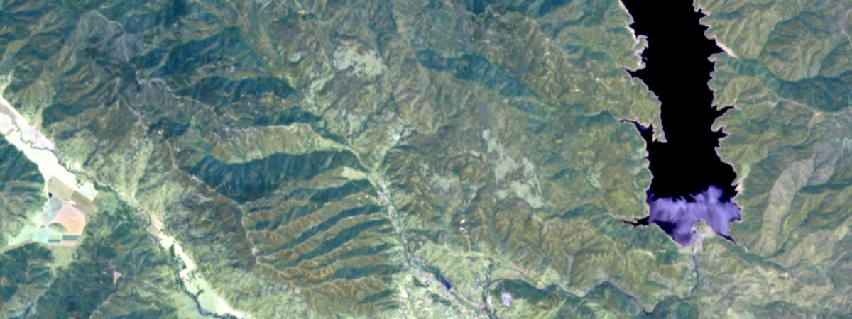
For comparison, the same area before the fire started shows no burn scar.
extract_band(prefire, [13,12,4])
Quantitative Assessment
The Normalized Burn Ratio (NBR) can be used to delineate the burnt areas and identify the severity of the fire.
The formula for the NBR is very similar to that of NDVI except that it uses near-infrared band 9 and the short-wave infrared band 13:
\begin{align}
{\mathbf{NBR}} = \frac{\mathbf{B9} - \mathbf{B13}}{\mathbf{B9} + \mathbf{B13} + \mathbf{WS}} \
\end{align}
The NBR equation was designed to be calcualted from reflectance, but it can be calculated from radiance and digitalnumber(dn) with changes to the burn severity table below. The WS parameter is used for water suppression, and is typically 2000.
For a given area, NBR is calculated from an image just prior to the burn and a second NBR is calculated for an image immediately following the burn. Burn extent and severity is judged by taking the difference between these two index layers:
\begin{align}
{\Delta \mathbf{NBR}} = \mathbf{NBR{prefire}} - \mathbf{NBR{postfire}} \
\end{align}
The meaning of the ∆NBR values can vary by scene, and interpretation in specific instances should always be based on some field assessment. However, the following table from the USGS FireMon program can be useful as a first approximation for interpreting the NBR difference:
| \begin{align}{\Delta \mathbf{NBR}} \end{align} | Burn Severity |
|---|---|
| 0.1 to 0.27 | Low severity burn |
| 0.27 to 0.44 | Medium severity burn |
| 0.44 to 0.66 | Moderate severity burn |
| > 0.66 | High severity burn |
[Source: http://wiki.landscapetoolbox.org/doku.php/remote_sensing_methods:normalized_burn_ratio]
Use Band Arithmetic and Map Algebra
In order to perform raster analysis on raw pixel value, we filter out the scenes from the sentinel image service again and create new layers
nbr_prefire  = band_arithmetic(prefire, "(b9 - b13) / (b9 + b13 + 2000)")
nbr_postfire = band_arithmetic(midfire, "(b9 - b13) / (b9 + b13 + 2000)")

nbr_diff = nbr_prefire - nbr_postfire
burnt_areas = colormap(remap(nbr_diff,
input_ranges=[0.1, 0.27, # low severity
0.27, 0.44, # medium severity
0.44, 0.66, # moderate severity
0.66, 1.00], # high severity burn
output_values=[1, 2, 3, 4],
no_data_ranges=[-1, 0.1], astype='u8'),
colormap=[[4, 0xFF, 0xC3, 0], [3, 0xFA, 0x8E, 0], [2, 0xF2, 0x55, 0], [1, 0xE6, 0, 0]])# Visualize burnt areas
burnt_areas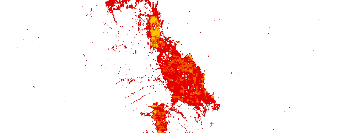
With this, we have computed the NBR on scenes from before and after the burn, and computed the NBR difference to identify places that have been affected by the fire. We've also normalized the values to match a burn severity index, and applied a color map that brings out the extent of fire damage.
Area calculation
pixx = (aoi['xmax'] - aoi['xmin']) / 1200.0
pixy = (aoi['ymax'] - aoi['ymin']) / 450.0

res = burnt_areas.compute_histograms(aoi, pixel_size={'x':pixx, 'y':pixy})

numpix = 0
histogram = res['histograms'][0]['counts'][1:]
for i in histogram:
    numpix += i
Report burnt area
sqmarea = numpix * pixx * pixy # in sq. m
acres = 0.00024711 * sqmarea   # in acres

HTML('<h3>Fire has consumed <font color="red">{:,} acres</font>  till {}</h3>.' \
     .format(int(acres), df.iloc[-1]['AcquisitionDate'].date()))
Fire has consumed
3,569 acres
till 2018-06-22.%matplotlib inline
plt.title('Distribution by severity', y=-0.1)
plt.pie(histogram, labels=['Low Severity', 'Medium Severity', 'Moderate Severity', 'High Severity']);
plt.axis('equal');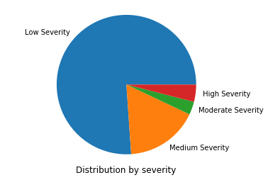
Visualize burnt areas
firemap = gis.map()
firemap.extent = aoi
firemap.add_layer([truecolor, burnt_areas])

firemap
Persist the burnt areas layer in the GIS
If required, using the save(), we can persist the output in the gis as a new layer. This uses distributed raster analysis to perform the analysis at the source resolution.
burnt_areas = burnt_areas.save()Raster to Feature layer conversion
Use Raster Analytics and Geoanalytics to convert the burnt area raster to a feature layer. The to_features() method converts the raster to a feature layer and create_buffers() fills holes in the features and dissolves them to output one feature that covers the extent of the Pawnee Fire.
burnt_areas = burnt_areas.layers[0]
fire_item = burnt_areas.to_features(output_name='Pawnee_Fire_Feature_Layer', gis=gis)
fire_layer = fire_item.layers[0]
fire = create_buffers(fire_layer, 100, 'Meters', dissolve_option='All', multipart=True, output_name='PawneeFireArea_Buffer')
fire = fire.layers[0]
Visualize Feature Layer
vectormap = gis.map()
vectormap.basemap = 'dark-gray'
vectormap.extent  = aoi

vectormap.add_layer(fire)
vectormap
Impact Assessment
Assess Human Impact
from arcgis import geometry

sdf = SpatialDataFrame.from_layer(fire)

fire_geometry = sdf.iloc[0].SHAPE
sa_filter = geometry.filters.intersects(geometry=fire_geometry, sr=4326)

def age_pyramid(df):
    %matplotlib inline
    warnings.simplefilter(action='ignore', category=FutureWarning)
    pd.options.mode.chained_assignment = None
    plt.style.use('ggplot')

    df = df[[x for x in impacted_people.columns if 'MALE' in x or 'FEM' in x]]
    sf = pd.DataFrame(df.sum())
    age = sf.index.str.extract('(\d+)').astype('int64')
    f = sf[sf.index.str.startswith('FEM')]
    m = sf[sf.index.str.startswith('MALE')]
    sf = sf.reset_index(drop = True)
    f = f.reset_index(drop = True)
    m = m.reset_index(drop = True)
    sf['age'] = age
    f["age"] = age
    m["age"] = age
    f = f.sort_values(by='age', ascending=False).set_index('age')
    m = m.sort_values(by='age', ascending=False).set_index('age')


    popdf = pd.concat([f, m], axis=1)
    popdf.columns = ['F', 'M']
    popdf['agelabel'] = popdf.index.map(str) + ' - ' + (popdf.index+4).map(str)
    popdf.M = -popdf.M

    sns.barplot(x="F", y="agelabel", color="#CC6699", label="Female", data=popdf, edgecolor='none')
    sns.barplot(x="M",  y="agelabel", color="#008AB8", label="Male",   data=popdf,  edgecolor='none')
    plt.ylabel('Age group')
    plt.xlabel('Number of people');
    return plt;
Age Pyramid of Affected Population
impacted_people = enrich(sdf, 'Age')
age_pyramid(impacted_people);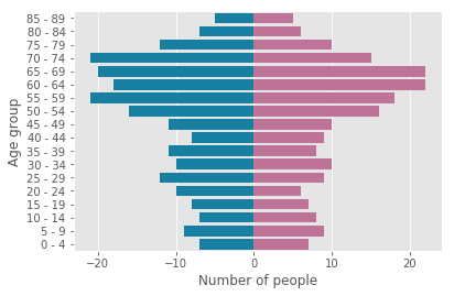
Conclusion
In this notebook example, we used Sentinel-2 data in order to perform remote sensing. For this we filtered out pre and post fire scenes. Using extract_band() we carried out visual assessment of the burnt area. We then computed the NBR on these scenes and computed the NBR difference to identify places that have been affected by the fire, using raster functions. We also normalized the values to match the burn severity index, applied a color map raster function that brings out the extent of fire damage and calculated the burnt area. Finally, we carried out a human impact assessment by plotting the age pyramid of affected population