Introduction
The arcgis.geoanalytics module provides types and functions for distributed analysis of large datasets. These GeoAnalytics tools work with big data registered in the GIS datastores as well as with feature layers.
In this notebook, we will go through the steps for setting up data to create a big data file share. We will also edit big data file share manifest to set spatial reference of the dataset. Once the data gets registered, we will demonstrate the utility of a number of tools including describe_dataset, aggregate_points, calculate_density, find_hot_spots, clip_layer, and run_python_script in order to better understand our data.
The sample aims to find answers to some fundamental questions:
- What is the spatial relationship between 911 calls?
- Which block groups have the highest number of 911 calls reporting?
- What is the most common reason for 911 calls?
- How many 911 calls occur each month?
- How many 911 calls occur each hour?
The data that will be used in this sample was originally obtained from data.gov open data portal. You can obtain data by searching using keywords, for example: 'Calls for Service New Orleans'. This sample demonstrates ability of ArcGIS API for Python to perform big data analysis on your infrastructure.
Note:
The ability to perform big data analysis is only available on ArcGIS Enterprise licensed with a GeoAnalytics server and not yet available on ArcGIS Online.
Necessary Imports
%matplotlib inline
import matplotlib.pyplot as plt
import pandas as pd
from datetime import datetime as dt

import arcgis
import arcgis.geoanalytics
from arcgis.gis import GIS

from arcgis.geoanalytics.summarize_data import aggregate_points, describe_dataset
from arcgis.geoanalytics.analyze_patterns import calculate_density, find_hot_spots
from arcgis.geoanalytics.manage_data import clip_layer, run_python_script
Connect to your ArcGIS Enterprise organization
gis = GIS('https://pythonapi.playground.esri.com/portal', 'arcgis_python', 'amazing_arcgis_123')Ensure your GIS supports GeoAnalytics
After connecting to Enterprise portal, we need to ensure an ArcGIS Enterprise GIS is set up with a licensed GeoAnalytics server. To do so, we will call the is_supported() method.
arcgis.geoanalytics.is_supported()True
Prepare the data
To register a file share or an HDFS, we need to format datasets as subfolders within a single parent folder and register the parent folder. This parent folder becomes a datastore, and each subfolder becomes a dataset. Our folder hierarchy would look like below:
|---FileShareFolder                 < -- The top-level folder is what is registered as a big data file share
   |---Calls                        < -- A folder "calls", composed of sub folders
      |---2011                      < -- A folder "2011", composed of 1 csv
         |---Calls_for_Service_2011.csv
      |---2012
         |---Calls_for_Service_2012.csv
      |---2013
         |---Calls_for_Service_2013.csv
      |---2014
         |---Calls_for_Service_2014.csv
      |---2015
         |---Calls_for_Service_2015.csv
      |---2016
         |---Calls_for_Service_2016.csv
      |---2017
         |---Calls_for_Service_2017.csv
      |---2018
         |---Calls_for_Service_2018.csv
      |---2019
         |---Calls_for_Service_2019.csv
Learn more about preparing your big data file share datasets here
Create a big data file share
The get_datastores() method of the geoanalytics module returns a DatastoreManager object that lets you search for and manage the big data file share items as Python API Datastore objects on your GeoAnalytics server.
bigdata_datastore_manager = arcgis.geoanalytics.get_datastores()
bigdata_datastore_manager
<DatastoreManager for https://pythonapi.playground.esri.com/ga/admin>
We will register service calls data as a big data file share using the add_bigdata() function on a DatastoreManager object.
When we register a directory, all subdirectories under the specified folder are also registered with the server. Always register the parent folder (for example, \machinename\mydatashare) that contains one or more individual dataset folders as the big data file share item. To learn more, see register a big data file share
Note: You cannot browse directories in ArcGIS Server Manager. You must provide the full path to the folder you want to register, for example, \myserver\share\bigdata. Avoid using local paths, such as C:\bigdata, unless the same data folder is available on all nodes of the server site.
# data_item = bigdata_datastore_manager.add_bigdata("ServiceCallsOrleans", r"\\machinename\datastore")Created Big Data file share for ServiceCallsOrleans
bigdata_fileshares = bigdata_datastore_manager.search(id='cff51a1a-4f27-4955-a3ef-5fa23240ccf9')
bigdata_fileshares
[<Datastore title:"/bigDataFileShares/ServiceCallsOrleans" type:"bigDataFileShare">]
file_share_folder = bigdata_fileshares[0]Once a big data file share is created, the GeoAnalytics server samples the datasets to generate a manifest, which outlines the data schema and specifies any time and geometry fields. A query of the resulting manifest returns each dataset's schema.. This process can take a few minutes depending on the size of your data. Once processed, querying the manifest property returns the schema of the datasets in your big data file share.
manifest = file_share_folder.manifest
manifest
{'datasets': [{'name': 'yearly_calls',
'format': {'quoteChar': '"',
'fieldDelimiter': ',',
'hasHeaderRow': True,
'encoding': 'UTF-8',
'escapeChar': '"',
'recordTerminator': '\n',
'type': 'delimited',
'extension': 'csv'},
'schema': {'fields': [{'name': 'NOPD_Item', 'type': 'esriFieldTypeString'},
{'name': 'Type_', 'type': 'esriFieldTypeString'},
{'name': 'TypeText', 'type': 'esriFieldTypeString'},
{'name': 'Priority', 'type': 'esriFieldTypeString'},
{'name': 'MapX', 'type': 'esriFieldTypeDouble'},
{'name': 'MapY', 'type': 'esriFieldTypeDouble'},
{'name': 'TimeCreate', 'type': 'esriFieldTypeString'},
{'name': 'TimeDispatch', 'type': 'esriFieldTypeString'},
{'name': 'TimeArrive', 'type': 'esriFieldTypeString'},
{'name': 'TimeClosed', 'type': 'esriFieldTypeString'},
{'name': 'Disposition', 'type': 'esriFieldTypeString'},
{'name': 'DispositionText', 'type': 'esriFieldTypeString'},
{'name': 'BLOCK_ADDRESS', 'type': 'esriFieldTypeString'},
{'name': 'Zip', 'type': 'esriFieldTypeBigInteger'},
{'name': 'PoliceDistrict', 'type': 'esriFieldTypeBigInteger'},
{'name': 'Location', 'type': 'esriFieldTypeString'}]},
'geometry': {'geometryType': 'esriGeometryPoint',
'spatialReference': {'wkid': 102682, 'latestWkid': 3452},
'fields': [{'name': 'MapX', 'formats': ['x']},
{'name': 'MapY', 'formats': ['y']}]},
'time': {'timeType': 'instant',
'timeReference': {'timeZone': 'UTC'},
'fields': [{'name': 'TimeCreate',
'formats': ['MM/dd/yyyy hh:mm:ss a']}]}}]}Edit a big data file share
The spatial reference of the dataset is set to 4326, but we know this data is from New Orleans, Louisiana, and is actually stored in the Louisiana State Plane Coordinate System. We need to edit the manifest with the correct spatial reference: {"wkid": 102682, "latestWkid": 3452}. Knowing the location where this data belongs to and the coordinate system which contains geospatial information of this dataset, we will edit our manifest. This will set the correct spatial reference.
manifest['datasets'][0]['geometry']['spatialReference'] = { "wkid": 102682, "latestWkid": 3452 }file_share_folder.manifest = manifestfile_share_folder.manifest{'datasets': [{'name': 'yearly_calls',
'format': {'quoteChar': '"',
'fieldDelimiter': ',',
'hasHeaderRow': True,
'encoding': 'UTF-8',
'escapeChar': '"',
'recordTerminator': '\n',
'type': 'delimited',
'extension': 'csv'},
'schema': {'fields': [{'name': 'NOPD_Item', 'type': 'esriFieldTypeString'},
{'name': 'Type_', 'type': 'esriFieldTypeString'},
{'name': 'TypeText', 'type': 'esriFieldTypeString'},
{'name': 'Priority', 'type': 'esriFieldTypeString'},
{'name': 'MapX', 'type': 'esriFieldTypeDouble'},
{'name': 'MapY', 'type': 'esriFieldTypeDouble'},
{'name': 'TimeCreate', 'type': 'esriFieldTypeString'},
{'name': 'TimeDispatch', 'type': 'esriFieldTypeString'},
{'name': 'TimeArrive', 'type': 'esriFieldTypeString'},
{'name': 'TimeClosed', 'type': 'esriFieldTypeString'},
{'name': 'Disposition', 'type': 'esriFieldTypeString'},
{'name': 'DispositionText', 'type': 'esriFieldTypeString'},
{'name': 'BLOCK_ADDRESS', 'type': 'esriFieldTypeString'},
{'name': 'Zip', 'type': 'esriFieldTypeBigInteger'},
{'name': 'PoliceDistrict', 'type': 'esriFieldTypeBigInteger'},
{'name': 'Location', 'type': 'esriFieldTypeString'}]},
'geometry': {'geometryType': 'esriGeometryPoint',
'spatialReference': {'wkid': 102682, 'latestWkid': 3452},
'fields': [{'name': 'MapX', 'formats': ['x']},
{'name': 'MapY', 'formats': ['y']}]},
'time': {'timeType': 'instant',
'timeReference': {'timeZone': 'UTC'},
'fields': [{'name': 'TimeCreate',
'formats': ['MM/dd/yyyy hh:mm:ss a']}]}}]}Get data for analysis
Search for big data file shares
Adding a big data file share to the Geoanalytics server adds a corresponding big data file share item on the portal. We can search for these types of items using the item_type parameter.
search_result = gis.content.search("bigDataFileShares_ServiceCallsOrleans", item_type = "big data file share", max_items=40)
search_result
[<Item title:"bigDataFileShares_ServiceCallsOrleans" type:Big Data File Share owner:portaladmin>]
data_item = search_result[0]data_item
Querying the layers property of the item returns a featureLayer representing the data. The object is actually an API Layer object.
data_item.layers[<Layer url:"https://pythonapi.playground.esri.com/ga/rest/services/DataStoreCatalogs/bigDataFileShares_ServiceCallsOrleans/BigDataCatalogServer/yearly_calls">]
calls = data_item.layers[0]calls.properties{
"dataStoreID": "cff51a1a-4f27-4955-a3ef-5fa23240ccf9",
"fields": [
{
"name": "NOPD_Item",
"type": "esriFieldTypeString"
},
{
"name": "Type_",
"type": "esriFieldTypeString"
},
{
"name": "TypeText",
"type": "esriFieldTypeString"
},
{
"name": "Priority",
"type": "esriFieldTypeString"
},
{
"name": "MapX",
"type": "esriFieldTypeDouble"
},
{
"name": "MapY",
"type": "esriFieldTypeDouble"
},
{
"name": "TimeCreate",
"type": "esriFieldTypeString"
},
{
"name": "TimeDispatch",
"type": "esriFieldTypeString"
},
{
"name": "TimeArrive",
"type": "esriFieldTypeString"
},
{
"name": "TimeClosed",
"type": "esriFieldTypeString"
},
{
"name": "Disposition",
"type": "esriFieldTypeString"
},
{
"name": "DispositionText",
"type": "esriFieldTypeString"
},
{
"name": "BLOCK_ADDRESS",
"type": "esriFieldTypeString"
},
{
"name": "Zip",
"type": "esriFieldTypeInteger"
},
{
"name": "PoliceDistrict",
"type": "esriFieldTypeInteger"
},
{
"name": "Location",
"type": "esriFieldTypeString"
}
],
"name": "yearly_calls",
"geometryType": "esriGeometryPoint",
"type": "featureClass",
"spatialReference": {
"wkid": 102682,
"latestWkid": 3452
},
"geometry": {
"fields": [
{
"name": "MapX",
"formats": [
"x"
]
},
{
"name": "MapY",
"formats": [
"y"
]
}
]
},
"time": {
"timeType": "instant",
"timeReference": {
"timeZone": "UTC"
},
"fields": [
{
"name": "TimeCreate",
"formats": [
"MM/dd/yyyy hh:mm:ss a"
]
}
]
},
"currentVersion": 10.81,
"children": []
}Search for feature layers
block_grp_item = gis.content.get('9975b4dd3ca24d4bbe6177b85f9da7bb')block_grp_itemWe will use the first item for our analysis. Since the item is a Feature Layer Collection, accessing the layers property will give us a list of Feature layer objects.
blk_grp_lyr = block_grp_item.layers[0]Describe data
The describe_dataset method provides an overview of big data. By default, the tool outputs a table layer containing calculated field statistics and a dict outlining geometry and time settings for the input layer.
Optionally, the tool can output a feature layer representing a sample set of features using the sample_size parameter, or a single polygon feature layer representing the input feature layers' extent by setting the extent_output parameter to True.
description = describe_dataset(input_layer=calls,
                               extent_output=True,
                               sample_size=1000,
                               output_name="Description of service calls" + str(dt.now().microsecond),
                               return_tuple=True)
{"messageCode":"BD_101051","message":"Possible issues were found while reading 'inputLayer'.","params":{"paramName":"inputLayer"}}
{"messageCode":"BD_101052","message":"Some records have either missing or invalid time values."}
{"messageCode":"BD_101054","message":"Some records have either missing or invalid geometries."}
description.output_json{'datasetName': 'calls',
'datasetSource': 'Big Data File Share - ServiceCallsOrleans',
'recordCount': 3952898,
'geometry': {'geometryType': 'Point',
'sref': {'wkid': 102682, 'latestWkid': 3452},
'countNonEmpty': 1763656,
'countEmpty': 2189242,
'spatialExtent': {'xmin': 0, 'ymin': 0, 'xmax': 37369000, 'ymax': 3513814}},
'time': {'timeType': 'Instant',
'countNonEmpty': 1763656,
'countEmpty': 2189242,
'temporalExtent': {'start': '2011-01-01 00:00:02.000',
'end': '2019-08-03 23:59:09.000'}}}description.sample_layer<FeatureLayer url:"https://deldevd014.esri.com/server/rest/services/Hosted/Description_of_service_calls223782/FeatureServer/2">
description.sample_layer.query().sdf| NOPD_Item | Type_ | TypeText | Priority | MapX | MapY | TimeCreate | TimeDispatch | TimeArrive | TimeClosed | Disposition | DispositionText | BLOCK_ADDRESS | Zip | PoliceDistrict | Location | INSTANT_DATETIME | globalid | OBJECTID | SHAPE | |
|---|---|---|---|---|---|---|---|---|---|---|---|---|---|---|---|---|---|---|---|---|
| 0 | A0247212 | 21 | COMPLAINT OTHER | 1H | 37369000.0 | 3513814.0 | 01/02/2012 05:16:04 PM | 01/02/2012 05:16:05 PM | 01/02/2012 05:16:05 PM | 01/02/2012 05:20:40 PM | NAT | NECESSARY ACTION TAKEN | 052XX N Claiborne Ave | NaN | 0.0 | (9.235500543E-7, -0.0000022929847665) | 2012-01-02 17:16:04 | {A471E188-9E41-2AA9-C46D-00771D78C616} | 12 | {'x': 1.8008574168558748e-05, 'y': 3.003918417... |
| 1 | L3180018 | 62A | BURGLAR ALARM, SILENT | 2E | NaN | NaN | 2E | 3706346 | 518681 | 12/25/2018 12:38:48 AM | 12/25/2018 12:42:11 AM | 12/25/2018 12:47:42 AM | 12/25/2018 12:58:28 AM | NaN | NaN | N | NaT | {8E68BDAF-E483-6952-ED6F-220A07FAEC2D} | 76 | None |
| 2 | H0789414 | 21 | COMPLAINT OTHER | 1H | 21.0 | NaN | 1H | 3671292 | 536599 | 08/06/2014 07:52:05 PM | None | 08/06/2014 07:52:05 PM | 08/06/2014 08:04:40 PM | NaN | NaN | Y | NaT | {003975B6-5491-DDB0-A0D8-6158F8EA62E0} | 133 | None |
| 3 | E3777812 | 62A | BURGLAR ALARM, SILEN | 2C | 3668023.0 | 517302.0 | 05/24/2012 12:47:03 PM | 05/24/2012 12:48:48 PM | 05/24/2012 12:51:46 PM | 05/24/2012 12:55:18 PM | NAT | NECESSARY ACTION TAKEN | 005XX Dufossat St | 70115.0 | 2.0 | (29.916803057765, -90.11110486281) | 2012-05-24 12:47:03 | {5ABCF635-D42E-92D4-3E1F-88F8853DCEC6} | 119 | {'x': -90.11111048458989, 'y': 29.916808462433... |
| 4 | I0820718 | 62A | BURGLAR ALARM, SILENT | 1A | NaN | NaN | 2E | 3704330 | 554832 | 09/07/2018 05:52:32 PM | 09/08/2018 12:52:59 AM | None | 09/08/2018 01:33:43 AM | NaN | NaN | N | NaT | {BC31F407-7C92-ADA5-5FFB-2B61E04604C2} | 114 | None |
| 5 | C1587515 | 21 | COMPLAINT OTHER | 1H | 21.0 | NaN | 1H | 3670550 | 539301 | 03/13/2015 09:42:20 PM | None | 03/13/2015 09:42:20 PM | 03/13/2015 09:53:24 PM | NaN | NaN | Y | NaT | {93EC1557-7D0A-539A-47A6-0EE7CEC9B645} | 126 | None |
| 6 | E0773819 | 107 | SUSPICIOUS PERSON | 2C | 3669625.0 | 532902.0 | 05/06/2019 09:07:17 AM | 05/06/2019 09:08:03 AM | 05/06/2019 09:10:27 AM | 05/06/2019 09:20:14 AM | GOA | GONE ON ARRIVAL | 107 | NaN | NaN | N | 2019-05-06 09:07:17 | {7BDE1FC8-733C-F08E-2624-A274A5E9AC61} | 172 | {'x': -90.10552626485547, 'y': 29.959656351679... |
| 7 | J3326816 | 21N | NOISE COMPLAINT | 1E | NaN | NaN | 1E | 3693027 | 535071 | 10/30/2016 06:00:21 AM | 10/30/2016 07:24:38 AM | 10/30/2016 07:33:03 AM | 10/30/2016 07:34:32 AM | NaN | NaN | N | NaT | {98B78BC8-4A35-0A0F-93E0-085E6490355C} | 278 | None |
| 8 | L4245411 | 62A | BURGLAR ALARM, SILEN | 2C | 3693800.0 | 525393.0 | 12/29/2011 04:47:02 PM | 12/29/2011 04:48:31 PM | 12/29/2011 04:56:36 PM | 12/29/2011 05:26:41 PM | NAT | NECESSARY ACTION TAKEN | 027XX Lawrence St | 70114.0 | 4.0 | (29.938269364881, -90.029451676433) | 2011-12-29 16:47:02 | {EC51B15E-98FD-B6A1-9905-412D09B336A6} | 187 | {'x': -90.02945727694797, 'y': 29.938274776870... |
| 9 | H1929011 | 103 | DISTURBANCE (OTHER) | 1C | 3679384.0 | 545506.0 | 08/13/2011 07:13:55 AM | 08/13/2011 07:13:57 AM | 08/13/2011 07:14:02 AM | 08/13/2011 07:17:31 AM | NAT | NECESSARY ACTION TAKEN | 015XX Sere St | 70122.0 | 3.0 | (29.994016435986, -90.074266619976) | 2011-08-13 07:13:55 | {976D05C0-6D29-2618-439B-678E9EB46D37} | 146 | {'x': -90.0742722350555, 'y': 29.9940218586582... |
| 10 | H0834814 | 21 | COMPLAINT OTHER | 1H | 21.0 | NaN | 1H | 3672670 | 540915 | 08/07/2014 03:43:05 AM | 08/07/2014 03:43:05 AM | 08/07/2014 04:13:10 AM | 08/07/2014 04:23:35 AM | NaN | NaN | N | NaT | {EBFC2284-8D11-B162-6801-CFB03ED6A7A9} | 206 | None |
| 11 | C2682218 | 103 | DISTURBANCE (OTHER) | 1A | 103.0 | NaN | 1C | 3687693 | 534738 | 03/22/2018 09:17:24 AM | 03/22/2018 09:31:34 AM | 03/22/2018 09:31:36 AM | 03/22/2018 10:10:04 AM | NaN | NaN | N | NaT | {0A9ED09A-EA2F-F7DB-9756-10173D9E76D7} | 305 | None |
| 12 | H1150317 | 17M | MUNICIPAL ATTACHMENT | 1F | 17.0 | NaN | 1G | 3670173 | 526285 | 08/09/2017 12:02:13 PM | None | 08/09/2017 12:02:13 PM | 08/09/2017 12:02:50 PM | NaN | NaN | Y | NaT | {ABED0474-C002-EE73-82AC-F48AE11AF6CF} | 311 | None |
| 13 | J3459717 | 21 | COMPLAINT OTHER | 1H | 67.0 | NaN | 1E | 3675387 | 534931 | 10/27/2017 07:26:01 PM | 10/28/2017 08:36:33 AM | 10/28/2017 08:36:49 AM | 10/28/2017 08:49:46 AM | NaN | NaN | N | NaT | {7197EBC3-81CC-03A3-6BAA-E3868DA10AB6} | 254 | None |
| 14 | E0116112 | 18 | TRAFFIC INCIDENT | 1H | 3697253.0 | 551601.0 | 05/01/2012 05:41:25 PM | 05/01/2012 05:41:25 PM | 05/01/2012 05:41:33 PM | 05/01/2012 06:09:18 PM | NAT | NECESSARY ACTION TAKEN | Chef Menteur Hwy & Stemway Dr | 70126.0 | 7.0 | (30.010223436348, -90.017600200365) | 2012-05-01 17:41:25 | {0B02A1FF-4259-F0E5-ADEB-F46F44BBA987} | 324 | {'x': -90.01760580074226, 'y': 30.010228864391... |
| 15 | I0860111 | 62A | BURGLAR ALARM, SILEN | 2C | 3680347.0 | 524357.0 | 09/07/2011 03:14:10 AM | 09/07/2011 03:16:26 AM | 09/07/2011 03:22:28 AM | 09/07/2011 03:27:41 AM | NAT | NECESSARY ACTION TAKEN | 014XX Magazine St | 70130.0 | 6.0 | (29.935834785662, -90.07196006635) | 2011-09-07 03:14:10 | {0213BAA0-A677-4003-E125-D7BE1ADB47FA} | 317 | {'x': -90.07196567831078, 'y': 29.935840195744... |
| 16 | B0297112 | 21 | COMPLAINT OTHER | 2H | 3692716.0 | 540389.0 | 02/02/2012 08:09:37 PM | 02/02/2012 08:43:07 PM | None | 02/02/2012 08:59:22 PM | NAT | NECESSARY ACTION TAKEN | 024XX Alvar St | 70117.0 | 5.0 | (29.979536989582, -90.032336408255) | 2012-02-02 20:09:37 | {3EB84BEC-4A5C-337A-98FB-FE7982255EF0} | 230 | {'x': -90.03234201131997, 'y': 29.979542410466... |
| 17 | I2182114 | 107 | SUSPICIOUS PERSON | 2A | 107.0 | NaN | 2A | 3681704 | 531287 | 09/17/2014 04:07:07 PM | None | 09/17/2014 04:07:07 PM | 09/17/2014 04:31:57 PM | NaN | NaN | Y | NaT | {5A1B7046-0DD3-F55B-81CB-90B9D6E333D4} | 258 | None |
| 18 | I3863213 | 18 | TRAFFIC INCIDENT | 1H | 3698925.0 | 557251.0 | 09/29/2013 04:01:05 AM | 09/29/2013 04:01:06 AM | 09/29/2013 04:01:05 AM | 09/29/2013 05:05:33 AM | NAT | Necessary Action Taken | I-10 W (7D04) & Morrison Rd Exit | 70126.0 | 7.0 | (30.025705895352, -90.012111936158) | 2013-09-29 04:01:05 | {E6F85E86-8803-7E4E-C2A9-5DD81C2950EA} | 525 | {'x': -90.01211753570936, 'y': 30.025711326943... |
| 19 | B0139512 | 21 | COMPLAINT OTHER | 1B | 3680623.0 | 525652.0 | 02/01/2012 08:53:09 PM | 02/01/2012 09:13:18 PM | None | 02/01/2012 09:32:21 PM | NAT | NECESSARY ACTION TAKEN | 011XX Erato St | 70130.0 | 6.0 | (29.939387249037, -90.071043691518) | 2012-02-01 20:53:09 | {089C1D47-D66A-040D-9164-9AE1C7DF1AFC} | 431 | {'x': -90.07104930338194, 'y': 29.939392659922... |
| 20 | F2337812 | 65 | SIMPLE ROBBERY | 1B | 3679940.0 | 529508.0 | 06/15/2012 11:20:15 PM | 06/15/2012 11:24:43 PM | 06/15/2012 11:41:09 PM | 06/16/2012 02:03:22 AM | RTF | REPORT TO FOLLOW | 005XX Baronne St | 70113.0 | 8.0 | (29.950010633457, -90.073066114888) | 2012-06-15 23:20:15 | {0AD4CBB9-E41A-8B1B-F89A-72387C6D4EDD} | 586 | {'x': -90.0730717277556, 'y': 29.9500160465899... |
| 21 | H1111512 | 21 | COMPLAINT OTHER | 1H | 3667387.0 | 534128.0 | 08/08/2012 12:24:12 AM | 08/08/2012 12:27:55 AM | 08/08/2012 12:28:55 AM | 08/08/2012 12:35:46 AM | NAT | NECESSARY ACTION TAKEN | 034XX S Carrollton Ave | 70125.0 | 2.0 | (29.963087783259, -90.11254651347) | 2012-08-08 00:24:12 | {CA58ACFE-54ED-B2F2-2454-3FFB9CA69437} | 563 | {'x': -90.11255213762003, 'y': 29.963093197957... |
| 22 | G1868016 | 59 | CRIMINAL MISCHIEF | 1F | 59.0 | NaN | 1F | 3667711 | 522588 | 07/17/2016 04:45:33 PM | None | None | 07/17/2016 06:10:49 PM | NaN | NaN | N | NaT | {B0995EEC-FE0D-6A05-92D8-DA61A3EC781F} | 518 | None |
| 23 | D3460315 | 20 | AUTO ACCIDENT | 1A | 20.0 | NaN | 1A | 3679962 | 526663 | 04/27/2015 06:25:27 PM | None | None | 04/27/2015 07:40:24 PM | NaN | NaN | N | NaT | {299E2EF4-E60B-2C56-919F-CB7DD65CFF2D} | 410 | None |
| 24 | H4376912 | 62A | BURGLAR ALARM, SILEN | 1C | 3681788.0 | 532676.0 | 08/28/2012 06:48:22 PM | 08/28/2012 07:19:29 PM | None | 08/28/2012 07:20:30 PM | NAT | NECESSARY ACTION TAKEN | 006XX Dauphine St | 70112.0 | 8.0 | (29.958665542329, -90.067120585039) | 2012-08-28 18:48:22 | {E1E36AC7-8FDD-0F08-23A6-C8D03FD7ECCE} | 613 | {'x': -90.0671261966614, 'y': 29.9586709575393... |
| 25 | A0451215 | 18 | TRAFFIC INCIDENT | 1H | 18.0 | NaN | 1H | 3697519 | 532902 | 01/05/2015 12:07:00 AM | 01/05/2015 12:07:00 AM | 01/05/2015 12:07:19 AM | 01/05/2015 12:17:43 AM | NaN | NaN | N | NaT | {6532C606-9BF6-097C-6620-CFDBC1B8FE20} | 514 | None |
| 26 | E2080514 | 21 | COMPLAINT OTHER | 1H | 21.0 | NaN | 1H | 3699489 | 555988 | 05/15/2014 08:40:26 PM | 05/15/2014 09:34:03 PM | None | 05/15/2014 09:36:27 PM | NaN | NaN | N | NaT | {48BBAFC2-6F72-F619-2C1A-005EC1643B9F} | 641 | None |
| 27 | K1291714 | 18 | TRAFFIC INCIDENT | 1H | 18.0 | NaN | 1H | 3674226 | 527339 | 11/11/2014 02:54:57 AM | None | 11/11/2014 02:54:57 AM | 11/11/2014 03:29:14 AM | NaN | NaN | Y | NaT | {E1FF75DD-BCF4-C9F0-DFC8-F98E886F986D} | 425 | None |
| 28 | J0065712 | 21 | COMPLAINT OTHER | 1H | 3681752.0 | 531382.0 | 10/01/2012 12:44:06 PM | 10/01/2012 12:44:27 PM | 10/01/2012 12:44:59 PM | 10/01/2012 12:52:25 PM | DUP | DUPLICATE | 003XX Royal St | 70130.0 | 8.0 | (29.955108575882, -90.067279411608) | 2012-10-01 12:44:06 | {77FCFBCA-49D8-A4B6-D8A5-822149E70D35} | 660 | {'x': -90.06728502312177, 'y': 29.955113990312... |
| 29 | E3786812 | 18 | TRAFFIC INCIDENT | 1H | 3683352.0 | 538374.0 | 05/24/2012 01:54:53 PM | 05/24/2012 01:54:53 PM | 05/24/2012 02:05:54 PM | 05/24/2012 02:24:43 PM | NAT | NECESSARY ACTION TAKEN | 018XX N Derbigny St | 70116.0 | 5.0 | (29.97428546205, -90.061982249162) | 2012-05-24 13:54:53 | {C9476A29-8114-D2BD-6FA3-9491B1FD736C} | 580 | {'x': -90.0619878600577, 'y': 29.9742908808282... |
| ... | ... | ... | ... | ... | ... | ... | ... | ... | ... | ... | ... | ... | ... | ... | ... | ... | ... | ... | ... | ... |
| 970 | L1621117 | 22A | AREA CHECK | 1I | NaN | NaN | 1I | 3671435 | 553142 | 12/14/2017 09:14:14 PM | 12/14/2017 09:14:14 PM | 12/14/2017 09:14:19 PM | 12/14/2017 09:38:10 PM | NaN | NaN | N | NaT | {C3A20D49-E44C-9717-CFA9-F2A5D47BCF9A} | 179 | None |
| 971 | H0552516 | 21 | COMPLAINT OTHER | 1H | 21.0 | NaN | 1H | 3692874 | 551918 | 08/05/2016 06:39:41 PM | None | 08/05/2016 06:39:41 PM | 08/05/2016 10:47:31 PM | NaN | NaN | Y | NaT | {5ECEE3CD-1712-9070-51DC-10790C55AE4A} | 196 | None |
| 972 | E0962512 | 17F | FUGITIVE ATTTACHMENT | 1G | 3684673.0 | 539982.0 | 05/06/2012 10:04:53 PM | 05/06/2012 10:04:53 PM | None | 05/06/2012 10:05:08 PM | RTF | REPORT TO FOLLOW | Elysian Fields Ave & N Galvez St | 70117.0 | 5.0 | (29.978666531583, -90.057753693797) | 2012-05-06 22:04:53 | {545A64C8-4872-3396-B99C-C524D5F56577} | 301 | {'x': -90.0577593037315, 'y': 29.9786719514519... |
| 973 | A3871913 | 18 | TRAFFIC INCIDENT | 1H | 3701559.0 | 516958.0 | 01/29/2013 01:26:56 PM | 01/29/2013 01:26:56 PM | 01/29/2013 01:26:58 PM | 01/29/2013 01:38:15 PM | NAT | NECESSARY ACTION TAKEN | General De Gaulle Dr & Huntlee D | 70131.0 | 4.0 | (29.914830976353, -90.005264597449) | 2013-01-29 13:26:56 | {EAD23CF8-07A5-AFB9-0643-8B8738F71A51} | 271 | {'x': -90.00527019039149, 'y': 29.914836384016... |
| 974 | I4080513 | 100 | HIT & RUN | 1E | 3660531.0 | 526542.0 | 09/30/2013 11:18:52 PM | 10/01/2013 02:04:05 AM | 10/01/2013 02:12:05 AM | 10/01/2013 02:16:20 AM | GOA | GONE ON ARRIVAL | 005XX S Carrollton Ave | 70118.0 | 2.0 | (29.942427784731, -90.134447707047) | 2013-09-30 23:18:52 | {0A9D4CC7-04E4-8CF7-C8B9-434F1C0E740A} | 272 | {'x': -90.134453336259, 'y': 29.94243319422235... |
| 975 | H3203611 | 62A | BURGLAR ALARM, SILEN | 2C | 3672373.0 | 518941.0 | 08/21/2011 08:38:09 AM | 08/21/2011 08:40:55 AM | 08/21/2011 08:42:33 AM | 08/21/2011 08:45:13 AM | NAT | NECESSARY ACTION TAKEN | 040XX Magazine St | 70115.0 | 6.0 | (29.921181484798, -90.097318619706) | 2011-08-21 08:38:09 | {BA45AE5B-03C8-E746-BE09-27E515EF1CE4} | 211 | {'x': -90.0973242379294, 'y': 29.9211868908671... |
| 976 | J1301516 | 103D | DOMESTIC DISTURBANCE | 2B | 35.0 | NaN | 2B | 3660930 | 531266 | 10/12/2016 04:28:05 PM | 10/12/2016 04:28:41 PM | 10/12/2016 04:37:15 PM | 10/12/2016 06:26:56 PM | NaN | NaN | N | NaT | {1E51063B-B2A2-73E3-4BDB-222AC9C1DA04} | 309 | None |
| 977 | L3766312 | 62A | BURGLAR ALARM, SILEN | 2C | 3701991.0 | 518152.0 | 12/27/2012 04:11:56 PM | 12/27/2012 04:15:28 PM | None | 12/27/2012 04:18:05 PM | VOI | VOID | 035XX Lang St | 70131.0 | 4.0 | (29.918100292854, -90.003857335737) | 2012-12-27 16:11:56 | {A0F02388-43F4-D44F-ECCE-28FC8EF2139E} | 297 | {'x': -90.00386292843632, 'y': 29.918105701276... |
| 978 | E0685114 | 18 | TRAFFIC INCIDENT | 1H | 18.0 | NaN | 1H | 3696210 | 551411 | 05/05/2014 11:30:29 PM | 05/05/2014 11:31:39 PM | 05/05/2014 11:30:29 PM | 05/05/2014 11:37:51 PM | NaN | NaN | Y | NaT | {BC5C4182-CC3A-50A2-7B39-BFB88A1E9D4E} | 372 | None |
| 979 | B1491111 | 107 | SUSPICIOUS PERSON | 2B | 3678129.0 | 533076.0 | 02/10/2011 12:45:04 PM | None | None | 02/10/2011 12:50:15 PM | DUP | DUPLICATE | 018XX Canal St | 70112.0 | 1.0 | (29.95987607933, -90.078660929549) | 2011-02-10 12:45:04 | {5A405527-7B44-78B0-3052-F3D52EB9C407} | 489 | {'x': -90.07866654435806, 'y': 29.959881494429... |
| 980 | I3344518 | 18 | TRAFFIC INCIDENT | 1J | 21.0 | NaN | 1J | 3698542 | 519147 | 09/27/2018 01:24:55 AM | 09/27/2018 01:24:55 AM | 09/27/2018 01:24:55 AM | 09/27/2018 02:03:41 AM | NaN | NaN | Y | NaT | {AF7F4840-037C-876F-557E-44ABDF216CAB} | 257 | None |
| 981 | E1886814 | 103 | DISTURBANCE (OTHER) | 2A | 103.0 | NaN | 2A | 3672223 | 525508 | 05/14/2014 03:23:26 PM | 05/14/2014 03:24:05 PM | 05/14/2014 03:34:00 PM | 05/14/2014 03:40:32 PM | NaN | NaN | N | NaT | {E585712D-C815-3258-5BB4-50FA9B3D93ED} | 347 | None |
| 982 | D1096317 | 62A | BURGLAR ALARM, SILENT | 1A | NaN | NaN | 2C | 3703440 | 560261 | 04/09/2017 09:05:17 PM | 04/10/2017 03:43:41 AM | None | 04/10/2017 04:10:19 AM | NaN | NaN | N | NaT | {212DA271-B29E-FF3F-18EF-6B2E453BFBB1} | 381 | None |
| 983 | J2543015 | 21 | COMPLAINT OTHER | 1H | NaN | NaN | 0E | 3675672 | 525857 | 10/21/2015 01:05:16 PM | 10/21/2015 01:10:01 PM | None | 10/21/2015 02:04:53 PM | NaN | NaN | N | NaT | {DC45D2C4-34FC-2213-9429-AC20AF027237} | 363 | None |
| 984 | G1014312 | 67 | THEFT | 1E | 3676106.0 | 530718.0 | 07/07/2012 03:21:21 PM | 07/07/2012 03:23:28 PM | 07/07/2012 03:23:33 PM | 07/07/2012 04:26:56 PM | RTF | REPORT TO FOLLOW | Bertrand St & Lafayette St | 70113.0 | 1.0 | (29.953453123323, -90.085130233788) | 2012-07-07 15:21:21 | {26FFD6F7-F70D-08E2-F5E8-89BC738AD6D8} | 416 | {'x': -90.08513585007961, 'y': 29.953458536814... |
| 985 | K3910518 | 22A | AREA CHECK | 1K | NaN | NaN | 1K | 3697581 | 515539 | 11/29/2018 08:07:55 PM | 11/29/2018 08:07:55 PM | 11/29/2018 08:07:55 PM | 11/29/2018 09:48:13 PM | NaN | NaN | Y | NaT | {8C8963FB-6638-252A-DE32-5281D6C5BD3D} | 403 | None |
| 986 | K1279211 | 21 | COMPLAINT OTHER | 1H | 37369000.0 | 3513814.0 | 11/09/2011 11:32:43 AM | 11/09/2011 11:34:39 AM | None | 11/09/2011 12:05:35 PM | NAT | NECESSARY ACTION TAKEN | 019XX Joann | NaN | 0.0 | (9.235500543E-7, -0.0000022929847665) | 2011-11-09 11:32:43 | {77A76953-7458-EE16-CFEF-7E50C18CE3D0} | 455 | {'x': 1.8008574168558748e-05, 'y': 3.003918417... |
| 987 | J2756411 | 99 | RECKLESS DRIVING | 2D | 3684064.0 | 547517.0 | 10/18/2011 10:30:47 PM | 10/18/2011 10:43:30 PM | None | 10/18/2011 10:47:35 PM | GOA | GONE ON ARRIVAL | Elysian Fields Ave & Gentilly Bl | 70122.0 | 3.0 | (29.999403737159, -90.059412555475) | 2011-10-18 22:30:47 | {41CB848F-2CD5-C099-F1E7-A24961015322} | 432 | {'x': -90.05941816675012, 'y': 29.999409161486... |
| 988 | I1844213 | 107 | SUSPICIOUS PERSON | 2A | 3679397.0 | 535828.0 | 09/14/2013 02:59:38 AM | 09/14/2013 03:03:08 AM | 09/14/2013 03:09:04 AM | 09/14/2013 03:15:08 AM | UNF | UNFOUNDED | 009XX N Prieur St | 70116.0 | 1.0 | (29.967404904189, -90.074561399733) | 2013-09-14 02:59:38 | {C61167EA-14E3-6246-2EB2-B964B6316807} | 521 | {'x': -90.07456701375169, 'y': 29.967410321060... |
| 989 | H1058117 | NOPD | INCIDENT REQUESTED BY ANOTHER AGENCY | 2A | NaN | NaN | 2A | 3696876 | 525312 | 08/08/2017 06:33:18 PM | None | None | 08/08/2017 06:33:59 PM | NaN | NaN | N | NaT | {D7847DCD-444D-AF11-8985-479601301C7D} | 741 | None |
| 990 | E2451818 | 58 | RETURN FOR ADDITIONAL INFO | 1I | 58.0 | NaN | 1I | 3672772 | 526264 | 05/19/2018 10:39:22 PM | 05/19/2018 10:39:22 PM | 05/19/2018 10:47:02 PM | 05/19/2018 11:16:59 PM | NaN | NaN | N | NaT | {24F27B84-3F54-B20E-9AFE-61F10AD7B8C8} | 543 | None |
| 991 | E2650811 | 67 | THEFT | 1E | 3677269.0 | 547605.0 | 05/17/2011 06:42:57 PM | 05/17/2011 07:50:41 PM | 05/17/2011 08:12:39 PM | 05/17/2011 10:00:51 PM | RTF | REPORT TO FOLLOW | 042XX Buchanan St | 70122.0 | 3.0 | (29.999851678873, -90.080875137137) | 2011-05-17 18:42:57 | {430BC094-3AA8-F5F3-F593-92697871071E} | 726 | {'x': -90.08088075426286, 'y': 29.999857102599... |
| 992 | H2357512 | 103 | DISTURBANCE (OTHER) | 1C | 3715565.0 | 564186.0 | 08/15/2012 04:49:19 PM | None | None | 08/15/2012 06:02:50 PM | VOI | VOID | 060XX Bullard Ave | 70128.0 | 7.0 | (30.044236292957, -89.959269638889) | 2012-08-15 16:49:19 | {5A3CC2E0-D43B-28ED-8BB4-49E9503A7EF0} | 630 | {'x': -89.95927522486834, 'y': 30.044241730303... |
| 993 | B0811515 | 21 | COMPLAINT OTHER | 1H | NaN | NaN | 0E | 3682795 | 525927 | 02/07/2015 04:07:46 PM | 02/07/2015 04:16:23 PM | None | 02/07/2015 04:22:03 PM | NaN | NaN | N | NaT | {0AB3B844-7776-83EB-04AD-AAAF9CD1C344} | 624 | None |
| 994 | E3981912 | 21 | COMPLAINT OTHER | 1H | 3682210.0 | 533199.0 | 05/25/2012 06:02:33 PM | 05/25/2012 06:02:33 PM | None | 05/25/2012 06:16:45 PM | NAT | NECESSARY ACTION TAKEN | Dauphine St & Saint Ann St | 70116.0 | 8.0 | (29.960090784609, -90.065769750523) | 2012-05-25 18:02:33 | {10D6A065-EE5B-A699-A0CB-136B7445DCC7} | 639 | {'x': -90.0657753618394, 'y': 29.9600962001742... |
| 995 | A2575219 | 22A | AREA CHECK | 1K | 3678685.0 | 536249.0 | 01/20/2019 08:44:04 AM | 01/20/2019 08:44:04 AM | 01/20/2019 08:44:04 AM | 01/20/2019 09:46:30 AM | NAT | Necessary Action Taken | 22A | NaN | NaN | Y | 2019-01-20 08:44:04 | {B4CF1985-73CB-398C-495C-EC752D62A62B} | 686 | {'x': -90.0768009430172, 'y': 29.9685894153133... |
| 996 | E2915114 | 17T | TRAFFIC ATTACHMENT | 1F | 17.0 | NaN | 1G | 3688424 | 540633 | 05/21/2014 08:34:25 PM | 05/21/2014 08:34:25 PM | None | 05/21/2014 08:34:37 PM | NaN | NaN | N | NaT | {23366D2E-DD2D-9306-F16B-FB396E542F75} | 651 | None |
| 997 | A0811415 | 62A | BURGLAR ALARM, SILENT | 2C | NaN | NaN | 2C | 3686861 | 541875 | 01/07/2015 10:39:22 PM | None | None | 01/07/2015 10:43:47 PM | NaN | NaN | N | NaT | {CA91D5A7-B617-960F-140E-70FA0D96A912} | 707 | None |
| 998 | L1133615 | 62C | SIMPLE BURGLARY VEHICLE | 1E | NaN | NaN | 1E | 3680642 | 537525 | 12/10/2015 01:21:07 PM | None | 12/10/2015 01:21:07 PM | 12/10/2015 01:52:47 PM | NaN | NaN | Y | NaT | {A1399702-B3FD-FB27-7D6F-649CCCD0F0F3} | 798 | None |
| 999 | B0108617 | 106 | OBSCENITY, EXPOSING | 2A | 106.0 | NaN | 2A | 3681317 | 530762 | 02/01/2017 08:14:41 PM | 02/01/2017 08:15:47 PM | 02/01/2017 08:15:53 PM | 02/02/2017 01:03:07 AM | NaN | NaN | N | NaT | {E13C6440-2B7D-A8AA-B7D4-A4923A84B8B5} | 764 | None |
1000 rows × 20 columns
We can see some records have missing or invalid attribute values, including in the fields the manifests defines as the time and geometry values. We will visualize a sample layer on the map to understand it better.
m1 = gis.map()
m1
m1.add_layer(description.sample_layer)The map shows that some data points have been located outside New Orleans because of missing or invalid geometries. We want to explore data points within New Orleans city limits. We will use clip_layer tool to extract only point features within the New Orleans boundary. This will remove data with missing or invalid geometries.
Extract features within New Orleans boundary
The clip_layer method extracts input point, line, or polygon features from an input_layer that fall within the boundaries of features in a clip_layer. The output layer contains a subset of features from the input layer. We will clip our input call feature layer to the New Orleans blk_grp_lyr features.
clip_result = clip_layer(calls, blk_grp_lyr, output_name="service calls in new Orleans" + str(dt.now().microsecond)){"messageCode":"BD_101051","message":"Possible issues were found while reading 'inputLayer'.","params":{"paramName":"inputLayer"}}
{"messageCode":"BD_101052","message":"Some records have either missing or invalid time values."}
{"messageCode":"BD_101054","message":"Some records have either missing or invalid geometries."}
clip_result
orleans_calls = clip_result.layers[0]m2 = gis.map("New Orleans")
m2
m2.add_layer(orleans_calls)Summarize data
We can use the aggregate_points method in the arcgis.geoanalytics.summarize_data submodule to group call features into individual block group features. The output polygon feature layer summarizes attribute information for all calls that fall within each block group. If no calls fall within a block group, that block group will not appear in the output.
The GeoAnalytics Tools use a process spatial reference during execution. Analyses with square or hexagon bins require a projected coordinate system. We'll use the World Cylindrical Equal Area projection (WKID 54034) below. All results are stored in the spatiotemporal datastore of the Enterprise in the WGS 84 Spatial Reference.
See the GeoAnalytics Documentation for a full explanation of analysis environment settings.
arcgis.env.process_spatial_reference = 54034agg_result = aggregate_points(orleans_calls,
polygon_layer=blk_grp_lyr,
output_name="aggregate results of call" + str(dt.now().microsecond))agg_resultm3 = gis.map("New Orleans")
m3
m3.add_layer(agg_result)m3.legend = TrueAnalyze patterns
The calculate_density method creates a density map from point features by spreading known quantities of some phenomenon (represented as attributes of the points) across the map. The result is a layer of areas classified from least dense to most dense. In this example, we will create density map by aggregating points within a bin of 1 kilometers. To learn more. please see here
cal_density = calculate_density(orleans_calls,
                                weight='Uniform',
                                bin_type='Square',
                                bin_size=1,
                                bin_size_unit="Kilometers",
                                time_step_interval=1,
                                time_step_interval_unit="Years",
                                time_step_repeat_interval=1,
                                time_step_repeat_interval_unit="Months",
                                time_step_reference=dt(2011, 1, 1),
                                radius=1000,
                                radius_unit="Meters",
                                area_units='SquareKilometers',
output_name="calculate density of call" + str(dt.now().microsecond))cal_densitym4 = gis.map("New Orleans")
m4
m4.add_layer(cal_density)m4.legend = TrueFind statistically significant hot and cold spots
The find_hot_spots tool analyzes point data and finds statistically significant spatial clustering of high (hot spots) and low (cold spots) numbers of incidents relative to the overall distribution of the data.
hot_spots = find_hot_spots(orleans_calls,
                           bin_size=100,
                           bin_size_unit='Meters',
                           neighborhood_distance=250,
                           neighborhood_distance_unit='Meters',
output_name="get hot spot areas" + str(dt.now().microsecond))hot_spotsm5 = gis.map("New Orleans")
m5
m5.add_layer(hot_spots)m5.legend = TrueThe darkest red features indicate areas where you can state with 99 percent confidence that the clustering of 911 call features is not the result of random chance but rather of some other variable that might be worth investigating. Similarly, the darkest blue features indicate that the lack of 911 calls is most likely not just random, but with 90% certainty you can state it is because of some variable in those locations. Features that are beige do not represent statistically significant clustering; the number of 911 calls could very likely be the result of random processes and random chance in those areas.
Visualize other aspects of data
The run_python_script method executes a Python script directly in an ArcGIS GeoAnalytics server site . The script can create an analysis pipeline by chaining together multiple GeoAnalytics tools without writing intermediate results to a data store. The tool can also distribute Python functionality across the GeoAnalytics server site.
Geoanalytics Server installs a Python 3.6 environment that this tool uses. The environment includes Spark 2.2.0, the compute platform that distributes analysis across multiple cores of one or more machines in your GeoAnalytics Server site. The environment includes the pyspark module which provides a collection of distributed analysis tools for data management, clustering, regression, and more. The run_python_script task automatically imports the pyspark module so you can directly interact with it.
When using the geoanalytics and pyspark packages, most functions return analysis results as Spark DataFrame memory structures. You can write these data frames to a data store or process them in a script. This lets you chain multiple geoanalytics and pyspark tools while only writing out the final result, eliminating the need to create any bulky intermediate result layers.
The TextType field contains the reason for the initial 911 call. Let's investigate the most frequent purposes for 911 calls in the New Orleans area by writing our own function:
def groupby_texttype():
    from datetime import datetime as dt
    # Calls data is stored in a feature service and accessed as a DataFrame via the layers object
    df = layers[0]
    # group the dataframe by TextType field and count the number of calls for each call type.
    out = df.groupBy('TypeText').count()
    # Write the final result to our datastore.
    out.write.format("webgis").save("groupby_texttype" + str(dt.now().microsecond))
In the fnction above, calls layer containing 911 call points is converted to a DataFrame. pyspark can used to group the dataframe by TypeText field to find the count of each category of call. The result can be saved as a feature service or other ArcGIS Enterprise layer type.
run_python_script(code=groupby_texttype, layers=[calls])[{'type': 'esriJobMessageTypeInformative',
'description': 'Executing (RunPythonScript): RunPythonScript "def groupby_texttype():\\n from datetime import datetime as dt\\n # Load the big data file share layer into a DataFrame.\\n df = layers[0]\\n # group the dataframe by TextType field and count the number of calls for each call type. \\n out = df.groupBy(\'TypeText\').count()\\n # Write the final result to our datastore.\\n output_name = "groupby_texttype" + str(dt.now().microsecond)\\n out.write.format("webgis").save(output_name)\\n\\ngroupby_texttype()" https://deldevd014.esri.com/server/rest/services/DataStoreCatalogs/bigDataFileShares_ServiceCallsOrleans/BigDataCatalogServer/calls "{"defaultAggregationStyles": false, "processSR": {"wkid": 54034}}"'},
{'type': 'esriJobMessageTypeInformative',
'description': 'Start Time: Mon Aug 26 15:03:57 2019'},
{'type': 'esriJobMessageTypeInformative',
'description': 'Using URL based GPRecordSet param: https://deldevd014.esri.com/server/rest/services/DataStoreCatalogs/bigDataFileShares_ServiceCallsOrleans/BigDataCatalogServer/calls'},
{'type': 'esriJobMessageTypeInformative',
'description': '{"messageCode":"BD_101028","message":"Starting new distributed job with 234 tasks.","params":{"totalTasks":"234"}}'},
{'type': 'esriJobMessageTypeInformative',
'description': '{"messageCode":"BD_101029","message":"0/234 distributed tasks completed.","params":{"completedTasks":"0","totalTasks":"234"}}'},
{'type': 'esriJobMessageTypeInformative',
'description': '{"messageCode":"BD_101029","message":"1/234 distributed tasks completed.","params":{"completedTasks":"1","totalTasks":"234"}}'},
{'type': 'esriJobMessageTypeInformative',
'description': '{"messageCode":"BD_101029","message":"5/234 distributed tasks completed.","params":{"completedTasks":"5","totalTasks":"234"}}'},
{'type': 'esriJobMessageTypeInformative',
'description': '{"messageCode":"BD_101029","message":"63/234 distributed tasks completed.","params":{"completedTasks":"63","totalTasks":"234"}}'},
{'type': 'esriJobMessageTypeInformative',
'description': '{"messageCode":"BD_101029","message":"234/234 distributed tasks completed.","params":{"completedTasks":"234","totalTasks":"234"}}'},
{'type': 'esriJobMessageTypeInformative',
'description': '{"messageCode":"BD_101081","message":"Finished writing results:"}'},
{'type': 'esriJobMessageTypeInformative',
'description': '{"messageCode":"BD_101082","message":"* Count of features = 283","params":{"resultCount":"283"}}'},
{'type': 'esriJobMessageTypeInformative',
'description': '{"messageCode":"BD_101083","message":"* Spatial extent = None","params":{"extent":"None"}}'},
{'type': 'esriJobMessageTypeInformative',
'description': '{"messageCode":"BD_101084","message":"* Temporal extent = None","params":{"extent":"None"}}'},
{'type': 'esriJobMessageTypeInformative',
'description': '{"messageCode":"BD_101226","message":"Feature service layer created: https://deldevd014.esri.com/server/rest/services/Hosted/groupby_texttype44974/FeatureServer/0","params":{"serviceUrl":"https://deldevd014.esri.com/server/rest/services/Hosted/groupby_texttype44974/FeatureServer/0"}}'},
{'type': 'esriJobMessageTypeInformative',
'description': 'Succeeded at Mon Aug 26 15:04:29 2019 (Elapsed Time: 31.45 seconds)'}]The result is saved as a feature layer. We can Search for the saved item using the search() method. Providing the search keyword same as the name we used for writing the result will retrieve the layer.
grp_cat = gis.content.search('groupby_texttype')[0]Accessing the tables property of the item will give us the tables object. We will then use query() method to read the table as spatially enabled dataframe.
grp_cat_df = grp_cat.tables[0].query().sdfSort the values in the decreasing order of the count field.
grp_cat_df.sort_values(by='count', ascending=False, inplace=True)grp_cat_df.head(10).plot(x='TypeText', y='count', kind='barh')<matplotlib.axes._subplots.AxesSubplot at 0x19fd0292898>
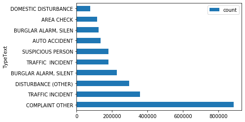
We can see that COMPLAINT OTHER is the most common category of call followed by TRAFFIC INCIDENTS.
Now we'll investigate 911 calls to investigate the most common reasons for calls within block addresses. We will define a new function to input to the run_python_script tool, this time grouping data by the TextType and BLOCK_ADDRESS attributes.
def grpby_cat_blkadd():
    from datetime import datetime as dt
    # Load the big data file share layer into a DataFrame
    df = layers[0]
    out = df.groupBy('TypeText', 'BLOCK_ADDRESS').count()
    out.write.format("webgis").save("grpby_cat_blkadd" + str(dt.now().microsecond))
run_python_script(code=grpby_cat_blkadd, layers=[calls])[{'type': 'esriJobMessageTypeInformative',
'description': 'Executing (RunPythonScript): RunPythonScript "def grpby_cat_blkadd():\\n from datetime import datetime as dt\\n # Load the big data file share layer into a DataFrame\\n df = layers[0]\\n out = df.groupBy(\'TypeText\', \'BLOCK_ADDRESS\').count()\\n out.write.format("webgis").save("grpby_cat_blkadd" + str(dt.now().microsecond))\\n\\ngrpby_cat_blkadd()" https://deldevd014.esri.com/server/rest/services/DataStoreCatalogs/bigDataFileShares_ServiceCallsOrleans/BigDataCatalogServer/calls "{"defaultAggregationStyles": false, "processSR": {"wkid": 54034}}"'},
{'type': 'esriJobMessageTypeInformative',
'description': 'Start Time: Mon Aug 26 15:17:49 2019'},
{'type': 'esriJobMessageTypeInformative',
'description': 'Using URL based GPRecordSet param: https://deldevd014.esri.com/server/rest/services/DataStoreCatalogs/bigDataFileShares_ServiceCallsOrleans/BigDataCatalogServer/calls'},
{'type': 'esriJobMessageTypeInformative',
'description': '{"messageCode":"BD_101028","message":"Starting new distributed job with 234 tasks.","params":{"totalTasks":"234"}}'},
{'type': 'esriJobMessageTypeInformative',
'description': '{"messageCode":"BD_101029","message":"0/234 distributed tasks completed.","params":{"completedTasks":"0","totalTasks":"234"}}'},
{'type': 'esriJobMessageTypeInformative',
'description': '{"messageCode":"BD_101029","message":"1/234 distributed tasks completed.","params":{"completedTasks":"1","totalTasks":"234"}}'},
{'type': 'esriJobMessageTypeInformative',
'description': '{"messageCode":"BD_101029","message":"7/234 distributed tasks completed.","params":{"completedTasks":"7","totalTasks":"234"}}'},
{'type': 'esriJobMessageTypeInformative',
'description': '{"messageCode":"BD_101029","message":"35/234 distributed tasks completed.","params":{"completedTasks":"35","totalTasks":"234"}}'},
{'type': 'esriJobMessageTypeInformative',
'description': '{"messageCode":"BD_101029","message":"82/234 distributed tasks completed.","params":{"completedTasks":"82","totalTasks":"234"}}'},
{'type': 'esriJobMessageTypeInformative',
'description': '{"messageCode":"BD_101029","message":"111/234 distributed tasks completed.","params":{"completedTasks":"111","totalTasks":"234"}}'},
{'type': 'esriJobMessageTypeInformative',
'description': '{"messageCode":"BD_101029","message":"161/234 distributed tasks completed.","params":{"completedTasks":"161","totalTasks":"234"}}'},
{'type': 'esriJobMessageTypeInformative',
'description': '{"messageCode":"BD_101029","message":"186/234 distributed tasks completed.","params":{"completedTasks":"186","totalTasks":"234"}}'},
{'type': 'esriJobMessageTypeInformative',
'description': '{"messageCode":"BD_101029","message":"234/234 distributed tasks completed.","params":{"completedTasks":"234","totalTasks":"234"}}'},
{'type': 'esriJobMessageTypeInformative',
'description': '{"messageCode":"BD_101081","message":"Finished writing results:"}'},
{'type': 'esriJobMessageTypeInformative',
'description': '{"messageCode":"BD_101082","message":"* Count of features = 2518651","params":{"resultCount":"2518651"}}'},
{'type': 'esriJobMessageTypeInformative',
'description': '{"messageCode":"BD_101083","message":"* Spatial extent = None","params":{"extent":"None"}}'},
{'type': 'esriJobMessageTypeInformative',
'description': '{"messageCode":"BD_101084","message":"* Temporal extent = None","params":{"extent":"None"}}'},
{'type': 'esriJobMessageTypeInformative',
'description': '{"messageCode":"BD_101226","message":"Feature service layer created: https://deldevd014.esri.com/server/rest/services/Hosted/grpby_cat_blkadd961138/FeatureServer/0","params":{"serviceUrl":"https://deldevd014.esri.com/server/rest/services/Hosted/grpby_cat_blkadd961138/FeatureServer/0"}}'},
{'type': 'esriJobMessageTypeInformative',
'description': 'Succeeded at Mon Aug 26 15:18:45 2019 (Elapsed Time: 56.25 seconds)'}]grp_cat_addr = gis.content.search('grpby_cat_blkadd')[0]grp_cat_addr_df = grp_cat_addr.tables[0].query().sdfgrp_cat_addr_df.sort_values(by='count', ascending=False, inplace=True)grp_cat_addr_df.head(10).plot(x='BLOCK_ADDRESS', y='count', kind='barh')<matplotlib.axes._subplots.AxesSubplot at 0x19fcff5f908>
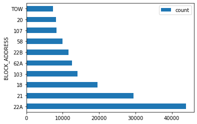
The chart shows that 22A block address has the highest number of incidents reported. So we want to further investigate the reason why this area had the most number of calls.
blk_addr_high = grp_cat_addr_df[grp_cat_addr_df['BLOCK_ADDRESS'] == '22A']blk_addr_high.head()| TypeText | BLOCK_ADDRESS | count | globalid | OBJECTID | |
|---|---|---|---|---|---|
| 2516001 | AREA CHECK | 22A | 43842 | {A703737A-EEF0-64D0-43A7-53BC43E0EEA1} | 2536366 |
| 2477875 | COMPLAINT OTHER | 22A | 147 | {4CE9300A-9C88-84F6-C19B-E63965844BAE} | 2478122 |
| 2477683 | BUSINESS CHECK | 22A | 119 | {DB15C4C7-1B57-4CB3-F3A5-2BA31DFE2AF1} | 2477922 |
| 2511367 | TRAFFIC INCIDENT | 22A | 60 | {9BA080BD-EE95-6A32-0483-82016B6FAE90} | 2521217 |
| 2513961 | DIRECTED PATROL | 22A | 34 | {0FAB1EB8-4524-9ECE-7AA6-3861770DEF10} | 2528186 |
blk_addr_high.TypeText.sort_values(ascending=False).head()1986885 WARR STOP WITH RELEASE 676774 WALKING BEAT 2036113 UNAUTHORIZED USE OF VEHICLE 649816 TRAFFIC INCIDENT 2226650 SUSPICIOUS PERSON Name: TypeText, dtype: object
The result indicates the most common reason for a 911 call in the 22A Block in New Orleans is defined as WARR STOP WITH RELEASE.
Now let's investigate the 911 call data for temporal trends. We saw in the manifest that the TimeCreate field holds specific time information for one instant (in UTC time zone) using a string format: MM/dd/yyyy hh:mm:ss a. We can parse these strings using Python's datetime module to extract year, month, day, hour, minute, and second to perform time analyses.
Let's define a helper function to convert the TimeCreate attribute field string types into a date type.
def calls_with_datetime():
    from datetime import datetime as dt
    # Load the big data file share layer into a DataFrame
    from pyspark.sql import functions as F
    df = layers[0]
    out = df.withColumn('datetime', F.unix_timestamp('TimeCreate', 'MM/dd/yyyy hh:mm:ss a').cast('timestamp'))
    out.write.format("webgis").save("calls_with_datetime" + str(dt.now().microsecond))
run_python_script(code=calls_with_datetime, layers=[calls])[{'type': 'esriJobMessageTypeInformative',
'description': 'Executing (RunPythonScript): RunPythonScript "def calls_with_datetime():\\n from datetime import datetime as dt\\n # Load the big data file share layer into a DataFrame\\n from pyspark.sql import functions as F\\n df = layers[0]\\n out = df.withColumn(\'datetime\', F.unix_timestamp(\'TimeCreate\', \'MM/dd/yyyy hh:mm:ss a\').cast(\'timestamp\'))\\n out.write.format("webgis").save("calls_with_datetime" + str(dt.now().microsecond))\\n\\ncalls_with_datetime()" https://deldevd014.esri.com/server/rest/services/DataStoreCatalogs/bigDataFileShares_ServiceCallsOrleans/BigDataCatalogServer/calls "{"defaultAggregationStyles": false, "processSR": {"wkid": 54034}}"'},
{'type': 'esriJobMessageTypeInformative',
'description': 'Start Time: Mon Aug 26 16:19:49 2019'},
{'type': 'esriJobMessageTypeInformative',
'description': 'Using URL based GPRecordSet param: https://deldevd014.esri.com/server/rest/services/DataStoreCatalogs/bigDataFileShares_ServiceCallsOrleans/BigDataCatalogServer/calls'},
{'type': 'esriJobMessageTypeInformative',
'description': '{"messageCode":"BD_101028","message":"Starting new distributed job with 34 tasks.","params":{"totalTasks":"34"}}'},
{'type': 'esriJobMessageTypeInformative',
'description': '{"messageCode":"BD_101029","message":"0/34 distributed tasks completed.","params":{"completedTasks":"0","totalTasks":"34"}}'},
{'type': 'esriJobMessageTypeInformative',
'description': '{"messageCode":"BD_101029","message":"1/34 distributed tasks completed.","params":{"completedTasks":"1","totalTasks":"34"}}'},
{'type': 'esriJobMessageTypeInformative',
'description': '{"messageCode":"BD_101029","message":"4/34 distributed tasks completed.","params":{"completedTasks":"4","totalTasks":"34"}}'},
{'type': 'esriJobMessageTypeInformative',
'description': '{"messageCode":"BD_101029","message":"5/34 distributed tasks completed.","params":{"completedTasks":"5","totalTasks":"34"}}'},
{'type': 'esriJobMessageTypeInformative',
'description': '{"messageCode":"BD_101029","message":"6/34 distributed tasks completed.","params":{"completedTasks":"6","totalTasks":"34"}}'},
{'type': 'esriJobMessageTypeInformative',
'description': '{"messageCode":"BD_101029","message":"9/34 distributed tasks completed.","params":{"completedTasks":"9","totalTasks":"34"}}'},
{'type': 'esriJobMessageTypeInformative',
'description': '{"messageCode":"BD_101029","message":"13/34 distributed tasks completed.","params":{"completedTasks":"13","totalTasks":"34"}}'},
{'type': 'esriJobMessageTypeInformative',
'description': '{"messageCode":"BD_101029","message":"24/34 distributed tasks completed.","params":{"completedTasks":"24","totalTasks":"34"}}'},
{'type': 'esriJobMessageTypeInformative',
'description': '{"messageCode":"BD_101029","message":"33/34 distributed tasks completed.","params":{"completedTasks":"33","totalTasks":"34"}}'},
{'type': 'esriJobMessageTypeInformative',
'description': '{"messageCode":"BD_101029","message":"34/34 distributed tasks completed.","params":{"completedTasks":"34","totalTasks":"34"}}'},
{'type': 'esriJobMessageTypeInformative',
'description': '{"messageCode":"BD_101081","message":"Finished writing results:"}'},
{'type': 'esriJobMessageTypeInformative',
'description': '{"messageCode":"BD_101082","message":"* Count of features = 3952898","params":{"resultCount":"3952898"}}'},
{'type': 'esriJobMessageTypeInformative',
'description': '{"messageCode":"BD_101083","message":"* Spatial extent = {\\"xmin\\":-101.51780476781194,\\"ymin\\":3.0039184174589957e-06,\\"xmax\\":1.8008574168558748e-05,\\"ymax\\":30.167660889419377}","params":{"extent":"{\\"xmin\\":-101.51780476781194,\\"ymin\\":3.0039184174589957e-06,\\"xmax\\":1.8008574168558748e-05,\\"ymax\\":30.167660889419377}"}}'},
{'type': 'esriJobMessageTypeInformative',
'description': '{"messageCode":"BD_101084","message":"* Temporal extent = Interval(MutableInstant(2011-01-01 00:00:02.000),MutableInstant(2019-08-03 23:59:09.000))","params":{"extent":"Interval(MutableInstant(2011-01-01 00:00:02.000),MutableInstant(2019-08-03 23:59:09.000))"}}'},
{'type': 'esriJobMessageTypeInformative',
'description': '{"messageCode":"BD_101226","message":"Feature service layer created: https://deldevd014.esri.com/server/rest/services/Hosted/calls_with_datetime470961/FeatureServer/0","params":{"serviceUrl":"https://deldevd014.esri.com/server/rest/services/Hosted/calls_with_datetime470961/FeatureServer/0"}}'},
{'type': 'esriJobMessageTypeInformative',
'description': 'Succeeded at Mon Aug 26 16:21:19 2019 (Elapsed Time: 1 minutes 29 seconds)'}]calls_with_datetime = gis.content.search('calls_with_datetime')[0]calls_with_datetime
calls_with_datetime_lyr = calls_with_datetime.layers[0]We will now split the date field into year, month and hour for studying temporal trends.
def call_with_added_date_time_cols():
    from datetime import datetime as dt
    # Load the big data file share layer into a DataFrame
    from pyspark.sql.functions import year, month, hour
    df = layers[0]
    df = df.withColumn('year', year(df['datetime']))
    df = df.withColumn('month', month(df['datetime']))
    out = df.withColumn('hour', hour(df['datetime']))
    out.write.format("webgis").save("call_with_added_date_time_cols" + str(dt.now().microsecond))
run_python_script(code=call_with_added_date_time_cols, layers=[calls_with_datetime_lyr])[{'type': 'esriJobMessageTypeInformative',
'description': 'Executing (RunPythonScript): RunPythonScript "def call_with_added_date_time_cols():\\n from datetime import datetime as dt\\n # Load the big data file share layer into a DataFrame\\n from pyspark.sql.functions import year, month, hour\\n df = layers[0]\\n df = df.withColumn(\'year\', year(df[\'datetime\']))\\n df = df.withColumn(\'month\', month(df[\'datetime\']))\\n out = df.withColumn(\'hour\', hour(df[\'datetime\']))\\n out.write.format("webgis").save("call_with_added_date_time_cols" + str(dt.now().microsecond))\\n\\ncall_with_added_date_time_cols()" https://deldevd014.esri.com/server/rest/services/Hosted/calls_with_datetime470961/FeatureServer/0 "{"defaultAggregationStyles": false, "processSR": {"wkid": 54034}}"'},
{'type': 'esriJobMessageTypeInformative',
'description': 'Start Time: Mon Aug 26 16:36:53 2019'},
{'type': 'esriJobMessageTypeInformative',
'description': 'Using URL based GPRecordSet param: https://deldevd014.esri.com/server/rest/services/Hosted/calls_with_datetime470961/FeatureServer/0'},
{'type': 'esriJobMessageTypeInformative',
'description': '{"messageCode":"BD_101028","message":"Starting new distributed job with 39 tasks.","params":{"totalTasks":"39"}}'},
{'type': 'esriJobMessageTypeInformative',
'description': '{"messageCode":"BD_101029","message":"0/39 distributed tasks completed.","params":{"completedTasks":"0","totalTasks":"39"}}'},
{'type': 'esriJobMessageTypeInformative',
'description': '{"messageCode":"BD_101029","message":"1/39 distributed tasks completed.","params":{"completedTasks":"1","totalTasks":"39"}}'},
{'type': 'esriJobMessageTypeInformative',
'description': '{"messageCode":"BD_101029","message":"5/39 distributed tasks completed.","params":{"completedTasks":"5","totalTasks":"39"}}'},
{'type': 'esriJobMessageTypeInformative',
'description': '{"messageCode":"BD_101029","message":"7/39 distributed tasks completed.","params":{"completedTasks":"7","totalTasks":"39"}}'},
{'type': 'esriJobMessageTypeInformative',
'description': '{"messageCode":"BD_101029","message":"14/39 distributed tasks completed.","params":{"completedTasks":"14","totalTasks":"39"}}'},
{'type': 'esriJobMessageTypeInformative',
'description': '{"messageCode":"BD_101029","message":"15/39 distributed tasks completed.","params":{"completedTasks":"15","totalTasks":"39"}}'},
{'type': 'esriJobMessageTypeInformative',
'description': '{"messageCode":"BD_101029","message":"20/39 distributed tasks completed.","params":{"completedTasks":"20","totalTasks":"39"}}'},
{'type': 'esriJobMessageTypeInformative',
'description': '{"messageCode":"BD_101029","message":"28/39 distributed tasks completed.","params":{"completedTasks":"28","totalTasks":"39"}}'},
{'type': 'esriJobMessageTypeInformative',
'description': '{"messageCode":"BD_101029","message":"35/39 distributed tasks completed.","params":{"completedTasks":"35","totalTasks":"39"}}'},
{'type': 'esriJobMessageTypeInformative',
'description': '{"messageCode":"BD_101029","message":"39/39 distributed tasks completed.","params":{"completedTasks":"39","totalTasks":"39"}}'},
{'type': 'esriJobMessageTypeInformative',
'description': '{"messageCode":"BD_101081","message":"Finished writing results:"}'},
{'type': 'esriJobMessageTypeInformative',
'description': '{"messageCode":"BD_101082","message":"* Count of features = 3952898","params":{"resultCount":"3952898"}}'},
{'type': 'esriJobMessageTypeInformative',
'description': '{"messageCode":"BD_101083","message":"* Spatial extent = {\\"xmin\\":-101.51780476781194,\\"ymin\\":3.0039184174589957e-06,\\"xmax\\":1.8008574168558748e-05,\\"ymax\\":30.167660889419377}","params":{"extent":"{\\"xmin\\":-101.51780476781194,\\"ymin\\":3.0039184174589957e-06,\\"xmax\\":1.8008574168558748e-05,\\"ymax\\":30.167660889419377}"}}'},
{'type': 'esriJobMessageTypeInformative',
'description': '{"messageCode":"BD_101084","message":"* Temporal extent = Interval(MutableInstant(2011-01-01 00:00:02.000),MutableInstant(2019-08-03 23:59:09.000))","params":{"extent":"Interval(MutableInstant(2011-01-01 00:00:02.000),MutableInstant(2019-08-03 23:59:09.000))"}}'},
{'type': 'esriJobMessageTypeInformative',
'description': '{"messageCode":"BD_101226","message":"Feature service layer created: https://deldevd014.esri.com/server/rest/services/Hosted/call_with_added_date_time_cols193397/FeatureServer/0","params":{"serviceUrl":"https://deldevd014.esri.com/server/rest/services/Hosted/call_with_added_date_time_cols193397/FeatureServer/0"}}'},
{'type': 'esriJobMessageTypeInformative',
'description': 'Succeeded at Mon Aug 26 16:40:14 2019 (Elapsed Time: 3 minutes 20 seconds)'}]date_time_added_item = gis.content.search('call_with_added_date_time_cols')date_time_added_item[0]date_time_added_lyr = date_time_added_item[0].layers[0]def grp_calls_by_month():
from datetime import datetime as dt
# Load the big data file share layer into a DataFrame
df = layers[0]
out = df.groupBy('month').count()
out.write.format("webgis").save("grp_calls_by_month" + str(dt.now().microsecond))run_python_script(code=grp_calls_by_month, layers=[date_time_added_lyr])[{'type': 'esriJobMessageTypeInformative',
'description': 'Executing (RunPythonScript): RunPythonScript "def grp_calls_by_month():\\n from datetime import datetime as dt\\n # Load the big data file share layer into a DataFrame\\n df = layers[0]\\n out = df.groupBy(\'month\').count()\\n out.write.format("webgis").save("grp_calls_by_month" + str(dt.now().microsecond))\\n\\ngrp_calls_by_month()" https://deldevd014.esri.com/server/rest/services/Hosted/call_with_added_date_time_cols193397/FeatureServer/0 "{"defaultAggregationStyles": false, "processSR": {"wkid": 54034}}"'},
{'type': 'esriJobMessageTypeInformative',
'description': 'Start Time: Mon Aug 26 16:40:16 2019'},
{'type': 'esriJobMessageTypeInformative',
'description': 'Using URL based GPRecordSet param: https://deldevd014.esri.com/server/rest/services/Hosted/call_with_added_date_time_cols193397/FeatureServer/0'},
{'type': 'esriJobMessageTypeInformative',
'description': '{"messageCode":"BD_101028","message":"Starting new distributed job with 239 tasks.","params":{"totalTasks":"239"}}'},
{'type': 'esriJobMessageTypeInformative',
'description': '{"messageCode":"BD_101029","message":"0/239 distributed tasks completed.","params":{"completedTasks":"0","totalTasks":"239"}}'},
{'type': 'esriJobMessageTypeInformative',
'description': '{"messageCode":"BD_101029","message":"1/239 distributed tasks completed.","params":{"completedTasks":"1","totalTasks":"239"}}'},
{'type': 'esriJobMessageTypeInformative',
'description': '{"messageCode":"BD_101029","message":"8/239 distributed tasks completed.","params":{"completedTasks":"8","totalTasks":"239"}}'},
{'type': 'esriJobMessageTypeInformative',
'description': '{"messageCode":"BD_101029","message":"9/239 distributed tasks completed.","params":{"completedTasks":"9","totalTasks":"239"}}'},
{'type': 'esriJobMessageTypeInformative',
'description': '{"messageCode":"BD_101029","message":"10/239 distributed tasks completed.","params":{"completedTasks":"10","totalTasks":"239"}}'},
{'type': 'esriJobMessageTypeInformative',
'description': '{"messageCode":"BD_101029","message":"12/239 distributed tasks completed.","params":{"completedTasks":"12","totalTasks":"239"}}'},
{'type': 'esriJobMessageTypeInformative',
'description': '{"messageCode":"BD_101029","message":"14/239 distributed tasks completed.","params":{"completedTasks":"14","totalTasks":"239"}}'},
{'type': 'esriJobMessageTypeInformative',
'description': '{"messageCode":"BD_101029","message":"16/239 distributed tasks completed.","params":{"completedTasks":"16","totalTasks":"239"}}'},
{'type': 'esriJobMessageTypeInformative',
'description': '{"messageCode":"BD_101029","message":"17/239 distributed tasks completed.","params":{"completedTasks":"17","totalTasks":"239"}}'},
{'type': 'esriJobMessageTypeInformative',
'description': '{"messageCode":"BD_101029","message":"19/239 distributed tasks completed.","params":{"completedTasks":"19","totalTasks":"239"}}'},
{'type': 'esriJobMessageTypeInformative',
'description': '{"messageCode":"BD_101029","message":"21/239 distributed tasks completed.","params":{"completedTasks":"21","totalTasks":"239"}}'},
{'type': 'esriJobMessageTypeInformative',
'description': '{"messageCode":"BD_101029","message":"23/239 distributed tasks completed.","params":{"completedTasks":"23","totalTasks":"239"}}'},
{'type': 'esriJobMessageTypeInformative',
'description': '{"messageCode":"BD_101029","message":"26/239 distributed tasks completed.","params":{"completedTasks":"26","totalTasks":"239"}}'},
{'type': 'esriJobMessageTypeInformative',
'description': '{"messageCode":"BD_101029","message":"35/239 distributed tasks completed.","params":{"completedTasks":"35","totalTasks":"239"}}'},
{'type': 'esriJobMessageTypeInformative',
'description': '{"messageCode":"BD_101029","message":"38/239 distributed tasks completed.","params":{"completedTasks":"38","totalTasks":"239"}}'},
{'type': 'esriJobMessageTypeInformative',
'description': '{"messageCode":"BD_101029","message":"239/239 distributed tasks completed.","params":{"completedTasks":"239","totalTasks":"239"}}'},
{'type': 'esriJobMessageTypeInformative',
'description': '{"messageCode":"BD_101081","message":"Finished writing results:"}'},
{'type': 'esriJobMessageTypeInformative',
'description': '{"messageCode":"BD_101082","message":"* Count of features = 13","params":{"resultCount":"13"}}'},
{'type': 'esriJobMessageTypeInformative',
'description': '{"messageCode":"BD_101083","message":"* Spatial extent = None","params":{"extent":"None"}}'},
{'type': 'esriJobMessageTypeInformative',
'description': '{"messageCode":"BD_101084","message":"* Temporal extent = None","params":{"extent":"None"}}'},
{'type': 'esriJobMessageTypeInformative',
'description': '{"messageCode":"BD_101226","message":"Feature service layer created: https://deldevd014.esri.com/server/rest/services/Hosted/grp_calls_by_month385803/FeatureServer/0","params":{"serviceUrl":"https://deldevd014.esri.com/server/rest/services/Hosted/grp_calls_by_month385803/FeatureServer/0"}}'},
{'type': 'esriJobMessageTypeInformative',
'description': 'Succeeded at Mon Aug 26 16:43:52 2019 (Elapsed Time: 3 minutes 36 seconds)'}]month = gis.content.search('grp_calls_by_month')[0]grp_month = month.tables[0]df_month = grp_month.query().sdfdf_month| month | count | globalid | OBJECTID | |
|---|---|---|---|---|
| 0 | 4.0 | 164835 | {B85CF9B6-A0B7-0CDB-2BD4-EE75CC1D8B7D} | 103 |
| 1 | 7.0 | 169707 | {9EDBD2EF-DC5E-FA4C-36B9-886AE09BEEB6} | 108 |
| 2 | 12.0 | 120340 | {F55F4B76-040A-B393-157B-84A13AA90D34} | 25 |
| 3 | 2.0 | 150248 | {1985235D-E1C1-F681-BDFC-4551A55A476A} | 175 |
| 4 | 9.0 | 120086 | {9F6CB958-8506-C6CD-13DC-7E39B13E1D02} | 90 |
| 5 | 6.0 | 165339 | {F51867CF-B370-11D7-106F-3BEA57712EAE} | 50 |
| 6 | 1.0 | 161162 | {667184E7-5446-EFC4-DF05-642A5F93B1C9} | 44 |
| 7 | 3.0 | 166684 | {24E0D747-1DF5-FB24-C5B5-4CACC874DB3B} | 52 |
| 8 | 5.0 | 171744 | {3BEDD3BF-726B-D044-5B75-FDF1D088FFFD} | 67 |
| 9 | NaN | 2189242 | {143D6439-ACBD-FD65-A324-1C26B8F7E75F} | 43 |
| 10 | 8.0 | 134547 | {B31419A6-0889-F609-E45E-B3506EDB07B7} | 104 |
| 11 | 10.0 | 124362 | {2E75CF98-AD0F-8F70-9F0C-83E89A5446F0} | 123 |
| 12 | 11.0 | 114602 | {077602D9-D33E-D51E-5657-3E0A823E1ABE} | 164 |
df_month.dropna().sort_values(by='month').plot(x='month', y='count', kind='bar')<matplotlib.axes._subplots.AxesSubplot at 0x19fd05de2e8>
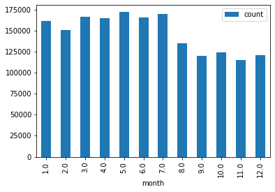
It shows that calls are most frequent in the earlier months of the year.
def grp_calls_by_hour():
    from datetime import datetime as dt
    # Load the big data file share layer into a DataFrame
    df = layers[0]
    out = df.groupBy('hour').count()
    out.write.format("webgis").save("grp_calls_by_hour" + str(dt.now().microsecond))
run_python_script(code=grp_calls_by_hour, layers=[date_time_added_lyr])[{'type': 'esriJobMessageTypeInformative',
'description': 'Executing (RunPythonScript): RunPythonScript "def grp_calls_by_hour():\\n from datetime import datetime as dt\\n # Load the big data file share layer into a DataFrame\\n df = layers[0]\\n out = df.groupBy(\'hour\').count()\\n out.write.format("webgis").save("grp_calls_by_hour" + str(dt.now().microsecond))\\n\\ngrp_calls_by_hour()" https://deldevd014.esri.com/server/rest/services/Hosted/call_with_added_date_time_cols193397/FeatureServer/0 "{"defaultAggregationStyles": false, "processSR": {"wkid": 54034}}"'},
{'type': 'esriJobMessageTypeInformative',
'description': 'Start Time: Mon Aug 26 16:49:37 2019'},
{'type': 'esriJobMessageTypeInformative',
'description': 'Using URL based GPRecordSet param: https://deldevd014.esri.com/server/rest/services/Hosted/call_with_added_date_time_cols193397/FeatureServer/0'},
{'type': 'esriJobMessageTypeInformative',
'description': '{"messageCode":"BD_101028","message":"Starting new distributed job with 239 tasks.","params":{"totalTasks":"239"}}'},
{'type': 'esriJobMessageTypeInformative',
'description': '{"messageCode":"BD_101029","message":"0/239 distributed tasks completed.","params":{"completedTasks":"0","totalTasks":"239"}}'},
{'type': 'esriJobMessageTypeInformative',
'description': '{"messageCode":"BD_101029","message":"1/239 distributed tasks completed.","params":{"completedTasks":"1","totalTasks":"239"}}'},
{'type': 'esriJobMessageTypeInformative',
'description': '{"messageCode":"BD_101029","message":"29/239 distributed tasks completed.","params":{"completedTasks":"29","totalTasks":"239"}}'},
{'type': 'esriJobMessageTypeInformative',
'description': '{"messageCode":"BD_101029","message":"239/239 distributed tasks completed.","params":{"completedTasks":"239","totalTasks":"239"}}'},
{'type': 'esriJobMessageTypeInformative',
'description': '{"messageCode":"BD_101081","message":"Finished writing results:"}'},
{'type': 'esriJobMessageTypeInformative',
'description': '{"messageCode":"BD_101082","message":"* Count of features = 25","params":{"resultCount":"25"}}'},
{'type': 'esriJobMessageTypeInformative',
'description': '{"messageCode":"BD_101083","message":"* Spatial extent = None","params":{"extent":"None"}}'},
{'type': 'esriJobMessageTypeInformative',
'description': '{"messageCode":"BD_101084","message":"* Temporal extent = None","params":{"extent":"None"}}'},
{'type': 'esriJobMessageTypeInformative',
'description': '{"messageCode":"BD_101226","message":"Feature service layer created: https://deldevd014.esri.com/server/rest/services/Hosted/grp_calls_by_hour873509/FeatureServer/0","params":{"serviceUrl":"https://deldevd014.esri.com/server/rest/services/Hosted/grp_calls_by_hour873509/FeatureServer/0"}}'},
{'type': 'esriJobMessageTypeInformative',
'description': 'Succeeded at Mon Aug 26 16:50:55 2019 (Elapsed Time: 1 minutes 18 seconds)'}]hour = gis.content.search('grp_calls_by_hour')[0]grp_hour = hour.tables[0]df_hour = grp_hour.query().sdfdf_hour.dropna().sort_values(by='hour').plot(x='hour', y='count', kind='bar')<matplotlib.axes._subplots.AxesSubplot at 0x19fd0ab4438>
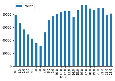
The chart above shows frequency of calls per hour of the day. We can see that there is a high frequency of calls during 4-5 p.m
Conclusion
We have shown spatial patterns in distribuition of emergency calls and the need of including temporal trends in the analysis. There is an obvious variation in the monthly, weekly, daily and even hourly distribution of service calls and this should be accounted for in further analysis or allocation of resources.