- Introduction
- Necessary Imports
- Connect to your ArcGIS Enterprise Organization
- Ensure your GIS supports GeoAnalytics
- Prepare the data
- Get data for analysis
- Describe data
- Analyze patterns
- Use Spark Dataframe and Run Python Script
- Conclusion
Introduction
Many of the poorest neighborhoods in the City of Chicago face violent crimes. With rapid increase in crime, amount of crime data is also increasing. Thus, there is a strong need to identify crime patterns in order to reduce its occurrence. Data mining using some of the most powerful tools available in ArcGIS API for Python is an effective way to analyze and detect patterns in data. Through this sample, we will demonstrate the utility of a number of geoanalytics tools including find_hot_spots, aggregate_points and calculate_density to visually understand geographical patterns.

The pyspark module available through run_python_script tool provides a collection of distributed analysis tools for data management, clustering, regression, and more. The run_python_script task automatically imports the pyspark module so you can directly interact with it. By calling this implementation of k-means in the run_python_script tool, we will cluster crime data into a predefined number of clusters. Such clusters are also useful in identifying crime patterns.
Further, based on the results of the analysis, the segmented crime map can be used to help efficiently dispatch officers throughout a city.
Necessary Imports
%matplotlib inline
import matplotlib.pyplot as plt
import pandas as pd
from datetime import datetime as dt

import arcgis
import arcgis.geoanalytics
from arcgis.gis import GIS
from arcgis.geoanalytics.summarize_data import describe_dataset, aggregate_points
from arcgis.geoanalytics.analyze_patterns import calculate_density, find_hot_spots
from arcgis.geoanalytics.manage_data import clip_layer, run_python_script
Connect to your ArcGIS Enterprise Organization
agol_gis = GIS('home')
gis = GIS('https://pythonapi.playground.esri.com/portal', 'arcgis_python', 'amazing_arcgis_123')
Ensure your GIS supports GeoAnalytics
Before executing a tool, we need to ensure an ArcGIS Enterprise GIS is set up with a licensed GeoAnalytics server. To do so, call the is_supported() method after connecting to your Enterprise portal. See the Components of ArcGIS URLs documentation for details on the urls to enter in the GIS parameters based on your particular Enterprise configuration.
arcgis.geoanalytics.is_supported()True
Prepare the data
To register a file share or an HDFS, we need to format datasets as subfolders within a single parent folder and register the parent folder. This parent folder becomes a datastore, and each subfolder becomes a dataset. Our folder hierarchy would look like below:

Learn more about preparing your big data file share datasets here.
Register a big data file share
The get_datastores() method of the geoanalytics module returns a DatastoreManager object that lets you search for and manage the big data file share items as Python API Datastore objects on your GeoAnalytics server.
bigdata_datastore_manager = arcgis.geoanalytics.get_datastores()
bigdata_datastore_manager
<DatastoreManager for https://pythonapi.playground.esri.com/ga/admin>
We will register chicago crime data as a big data file share using the add_bigdata() function on a DatastoreManager object.
When we register a directory, all subdirectories under the specified folder are also registered with the server. Always register the parent folder (for example, \machinename\mydatashare) that contains one or more individual dataset folders as the big data file share item. To learn more, see register a big data file share.
Note: You cannot browse directories in ArcGIS Server Manager. You must provide the full path to the folder you want to register, for example, \myserver\share\bigdata. Avoid using local paths, such as C:\bigdata, unless the same data folder is available on all nodes of the server site.
# data_item = bigdata_datastore_manager.add_bigdata("Chicago_Crime_2001_2020", r"\\machine_name\data\chicago")Created Big Data file share for Chicago_Crime_2001_2020
bigdata_fileshares = bigdata_datastore_manager.search(id='0e7a861d-c1c5-4acc-869d-05d2cebbdbee')
bigdata_fileshares
[<Datastore title:"/bigDataFileShares/GA_Data" type:"bigDataFileShare">]
file_share_folder = bigdata_fileshares[0]Once a big data file share is created, the GeoAnalytics server samples the datasets to generate a manifest, which outlines the data schema and specifies any time and geometry fields. A query of the resulting manifest returns each dataset's schema. This process can take a few minutes depending on the size of your data. Once processed, querying the manifest property returns the schema of the datasets in your big data file share.
manifest = file_share_folder.manifest['datasets'][1]
manifest
{'name': 'crime',
'format': {'quoteChar': '"',
'fieldDelimiter': ',',
'hasHeaderRow': True,
'encoding': 'UTF-8',
'escapeChar': '"',
'recordTerminator': '\n',
'type': 'delimited',
'extension': 'csv'},
'schema': {'fields': [{'name': 'ID', 'type': 'esriFieldTypeBigInteger'},
{'name': 'Case Number', 'type': 'esriFieldTypeString'},
{'name': 'Date', 'type': 'esriFieldTypeString'},
{'name': 'Block', 'type': 'esriFieldTypeString'},
{'name': 'IUCR', 'type': 'esriFieldTypeString'},
{'name': 'Primary Type', 'type': 'esriFieldTypeString'},
{'name': 'Description', 'type': 'esriFieldTypeString'},
{'name': 'Location Description', 'type': 'esriFieldTypeString'},
{'name': 'Arrest', 'type': 'esriFieldTypeString'},
{'name': 'Domestic', 'type': 'esriFieldTypeString'},
{'name': 'Beat', 'type': 'esriFieldTypeBigInteger'},
{'name': 'District', 'type': 'esriFieldTypeBigInteger'},
{'name': 'Ward', 'type': 'esriFieldTypeBigInteger'},
{'name': 'Community Area', 'type': 'esriFieldTypeBigInteger'},
{'name': 'FBI Code', 'type': 'esriFieldTypeString'},
{'name': 'X Coordinate', 'type': 'esriFieldTypeBigInteger'},
{'name': 'Y Coordinate', 'type': 'esriFieldTypeBigInteger'},
{'name': 'Year', 'type': 'esriFieldTypeBigInteger'},
{'name': 'Updated On', 'type': 'esriFieldTypeString'},
{'name': 'Latitude', 'type': 'esriFieldTypeDouble'},
{'name': 'Longitude', 'type': 'esriFieldTypeDouble'},
{'name': 'Location', 'type': 'esriFieldTypeString'}]},
'geometry': {'geometryType': 'esriGeometryPoint',
'spatialReference': {'wkid': 4326},
'fields': [{'name': 'Location', 'formats': ['({y},{x})']}]},
'time': {'timeType': 'instant',
'timeReference': {'timeZone': 'UTC'},
'fields': [{'name': 'Date', 'formats': ['MM/dd/yyyy hh:mm:ss a']}]}}Get data for analysis
Adding a big data file share to the Geoanalytics server adds a corresponding big data file share item on the portal. We can search for these types of items using the item_type parameter.
search_result = gis.content.search("bigDataFileShares_GA_Data", item_type = "big data file share")
search_result
[<Item title:"bigDataFileShares_GA_Data" type:Big Data File Share owner:arcgis_python>]
ga_item = search_result[0]ga_item
Querying the layers property of the item returns a featureLayer representing the data. The object is actually an API Layer object.
ga_item.layers[<Layer url:"https://pythonapi.playground.esri.com/ga/rest/services/DataStoreCatalogs/bigDataFileShares_GA_Data/BigDataCatalogServer/air_quality">, <Layer url:"https://pythonapi.playground.esri.com/ga/rest/services/DataStoreCatalogs/bigDataFileShares_GA_Data/BigDataCatalogServer/crime">, <Layer url:"https://pythonapi.playground.esri.com/ga/rest/services/DataStoreCatalogs/bigDataFileShares_GA_Data/BigDataCatalogServer/calls">, <Layer url:"https://pythonapi.playground.esri.com/ga/rest/services/DataStoreCatalogs/bigDataFileShares_GA_Data/BigDataCatalogServer/analyze_new_york_city_taxi_data">]
crime_lyr = ga_item.layers[1]illinois_blk_grps = agol_gis.content.get('a11d886be35149cb9dab0f7aac75a2af')illinois_blk_grps
blk_lyr = illinois_blk_grps.layers[0]We will filter the blockgroups by 031 code which is county code for Chicago.
blk_lyr.filter = "COUNTYFP = '031'"m2 = gis.map('chicago')
m2
m2.add_layer(blk_lyr)Describe data
The describe_dataset method provides an overview of big data. By default, the tool outputs a table layer containing calculated field statistics and a dict outlining geometry and time settings for the input layer.
Optionally, the tool can output a feature layer representing a sample set of features using the sample_size parameter, or a single polygon feature layer representing the input feature layers' extent by setting the extent_output parameter to True.
description = describe_dataset(input_layer=crime_lyr,
                               extent_output=True,
                               sample_size=1000,
                               output_name="Description of crime data" + str(dt.now().microsecond),
return_tuple=True)description.output_json{'datasetName': 'crime',
'datasetSource': 'Big Data File Share - Chicago_Crime_2001_2020',
'recordCount': 7061128,
'geometry': {'geometryType': 'Point',
'sref': {'wkid': 4326},
'countNonEmpty': 6993512,
'countEmpty': 67616,
'spatialExtent': {'xmin': -91.686565684,
'ymin': 36.619446395,
'xmax': -87.524529378,
'ymax': 42.022910333}},
'time': {'timeType': 'Instant',
'countNonEmpty': 7061128,
'countEmpty': 67616,
'temporalExtent': {'start': '2001-01-01 00:00:00.000',
'end': '2020-01-26 23:40:00.000'}}}sdf_desc_output = description.output.query(as_df=True)
sdf_desc_output.head()| FIELD_NAME | COUNT | COUNT_NON_EMPTY | AVG | MIN | MAX | STDDEV | RANGE | SUM | VAR | ANY | globalid | OBJECTID | |
|---|---|---|---|---|---|---|---|---|---|---|---|---|---|
| 0 | ID | 7061128 | 7061128 | 6.468796e+06 | 634.0 | 11969378.0 | 3.180550e+06 | 11968744.0 | 4.567699e+13 | 1.011590e+13 | None | {46B95A04-F3C3-FA20-D745-B2C7C9E7AFAF} | 1 |
| 1 | Case Number | 7061128 | 7061124 | NaN | NaN | NaN | NaN | NaN | NaN | NaN | JD114742 | {7FCBD37F-459C-E78F-B873-CA734429AA9B} | 2 |
| 2 | Date | 7061128 | 7061128 | NaN | NaN | NaN | NaN | NaN | NaN | NaN | 01/01/2001 12:00:00 AM | {A7E0431E-0AD4-EC59-38A9-F71177ACDF45} | 3 |
| 3 | Block | 7061128 | 7061128 | NaN | NaN | NaN | NaN | NaN | NaN | NaN | 061XX S FAIRFIELD AVE | {FF3E7A5E-A887-D815-7812-AD995620C5A9} | 4 |
| 4 | IUCR | 7061128 | 6761589 | 1.127044e+03 | 110.0 | 9901.0 | 8.126368e+02 | 9791.0 | 7.620611e+09 | 6.603785e+05 | None | {3A5F5858-F0FD-932D-DF6D-FF8355F9141B} | 5 |
description.sample_layer<FeatureLayer url:"https://ndhagsb01.esri.com/gis/rest/services/Hosted/Description_of_crime_data956049/FeatureServer/2">
sdf_slyr = description.sample_layer.query(as_df=True)
sdf_slyr.head()| ID | Case_Number | Date | Block | IUCR | Primary_Type | Description | Location_Description | Arrest | Domestic | ... | Y_Coordinate | Year | Updated_On | Latitude | Longitude | Location | INSTANT_DATETIME | globalid | OBJECTID | SHAPE | |
|---|---|---|---|---|---|---|---|---|---|---|---|---|---|---|---|---|---|---|---|---|---|
| 0 | 8196694 | HT430829 | 08/04/2011 02:10:00 AM | 079XX S MERRILL AVE | 520.0 | ASSAULT | AGGRAVATED:KNIFE/CUTTING INSTR | RESIDENCE | true | false | ... | 1852704.0 | 2011 | 02/10/2018 03:50:01 PM | 41.750809 | -87.572309 | (41.750808511, -87.572308641) | 2011-08-04 02:10:00 | {25BA0BFD-A32B-802A-72C5-D8A698A3C06F} | 1 | {'x': -87.572308641, 'y': 41.750808511, 'spati... |
| 1 | 5139385 | HM736684 | 11/22/2006 09:00:00 PM | 019XX N MOHAWK ST | 1310.0 | CRIMINAL DAMAGE | TO PROPERTY | OTHER | false | false | ... | 1913191.0 | 2006 | 02/10/2018 03:50:01 PM | 41.917244 | -87.642423 | (41.917243909, -87.642422501) | 2006-11-22 21:00:00 | {A67F0D22-7EED-03EE-511A-49458AB189C7} | 2 | {'x': -87.642422501, 'y': 41.917243909, 'spati... |
| 2 | 6257174 | HP338636 | 05/16/2008 05:30:00 AM | 108XX S LOWE AVE | 915.0 | MOTOR VEHICLE THEFT | TRUCK, BUS, MOTOR HOME | STREET | false | false | ... | 1832936.0 | 2008 | 02/28/2018 03:56:25 PM | 41.696981 | -87.638886 | (41.696980545, -87.638886196) | 2008-05-16 05:30:00 | {5FE25286-201F-EF1D-3D6F-ECF7AC8DA402} | 3 | {'x': -87.638886196, 'y': 41.696980545, 'spati... |
| 3 | 8518985 | HV195817 | 01/20/2012 09:00:00 AM | 047XX S KNOX AVE | 840.0 | THEFT | FINANCIAL ID THEFT: OVER $300 | RESIDENCE | false | false | ... | 1872783.0 | 2012 | 02/10/2018 03:50:01 PM | 41.806897 | -87.739467 | (41.806896849, -87.739466549) | 2012-01-20 09:00:00 | {F475734C-7CC7-06DC-75F3-B1D9D6D91D8E} | 4 | {'x': -87.739466549, 'y': 41.806896849, 'spati... |
| 4 | 3930218 | HL301854 | 04/17/2005 11:40:00 PM | 039XX W ARMITAGE AVE | 1220.0 | DECEPTIVE PRACTICE | THEFT OF LOST/MISLAID PROP | ALLEY | true | false | ... | 1912994.0 | 2005 | 02/28/2018 03:56:25 PM | 41.917175 | -87.725912 | (41.917175309, -87.725912468) | 2005-04-17 23:40:00 | {862B9571-2761-454E-56E4-F19124DCC584} | 5 | {'x': -87.725912468, 'y': 41.917175309, 'spati... |
5 rows × 26 columns
m1 = gis.map('chicago')
m1
m1.add_layer(description.sample_layer)m1.legend = TrueAnalyze patterns
The GeoAnalytics Tools use a process spatial reference during execution. Analyses with square or hexagon bins require a projected coordinate system. We'll use 26771 as seen from http://epsg.io/?q=illinois%20kind%3APROJCRS.
arcgis.env.process_spatial_reference = 26771 Aggregate points
We can use the aggregate_points method in the arcgis.geoanalytics.summarize_data submodule to group call features into individual block group features. The output polygon feature layer summarizes attribute information for all calls that fall within each block group. If no calls fall within a block group, that block group will not appear in the output.
The GeoAnalytics Tools use a process spatial reference during execution. Analyses with square or hexagon bins require a projected coordinate system. We'll use the World Cylindrical Equal Area projection (WKID 54034) below. All results are stored in the spatiotemporal datastore of the Enterprise in the WGS 84 Spatial Reference.
See the GeoAnalytics Documentation for a full explanation of analysis environment settings.
agg_result = aggregate_points(crime_lyr,
                              polygon_layer=blk_lyr,
                              output_name="aggregate results of crime" + str(dt.now().microsecond))
{"messageCode":"BD_101189","message":"The GeoAnalytics job is waiting for resources and has not started yet. The job will automatically cancel after 10 minutes.","params":{"minutes":"10"}}
{"messageCode":"BD_101189","message":"The GeoAnalytics job is waiting for resources and has not started yet. The job will automatically cancel after 10 minutes.","params":{"minutes":"10"}}
{"messageCode":"BD_101051","message":"Possible issues were found while reading 'pointLayer'.","params":{"paramName":"pointLayer"}}
{"messageCode":"BD_101054","message":"Some records have either missing or invalid geometries."}
agg_result
m3 = gis.map('chicago')
m3
m3.add_layer(agg_result)m3.legend = TrueCalculate density
The calculate_density method creates a density map from point features by spreading known quantities of some phenomenon (represented as attributes of the points) across the map. The result is a layer of areas classified from least dense to most dense. In this example, we will create density map by aggregating points within a bin of 1 kilometer. To learn more. please see here.
cal_density = calculate_density(crime_lyr,
                                weight='Uniform',
                                bin_type='Square',
                                bin_size=1,
                                bin_size_unit="Kilometers",
                                time_step_interval=1,
                                time_step_interval_unit="Years",
                                time_step_repeat_interval=1,
                                time_step_repeat_interval_unit="Months",
                                time_step_reference=dt(2001, 1, 1),
                                radius=1000,
                                radius_unit="Meters",
                                area_units='SquareKilometers',
                                output_name="calculate density of crime" + str(dt.now().microsecond))
{"messageCode":"BD_101051","message":"Possible issues were found while reading 'inputLayer'.","params":{"paramName":"inputLayer"}}
{"messageCode":"BD_101054","message":"Some records have either missing or invalid geometries."}
m4 = gis.map('chicago')
m4
m4.add_layer(cal_density)m4.legend = TrueThe find_hot_spots tool analyzes point data and finds statistically significant spatial clustering of high (hot spots) and low (cold spots) numbers of incidents relative to the overall distribution of the data.
Find hot spots
The find_hot_spots tool analyzes point data and finds statistically significant spatial clustering of high (hot spots) and low (cold spots) numbers of incidents relative to the overall distribution of the data.
hot_spots = find_hot_spots(crime_lyr,
                           bin_size=100,
                           bin_size_unit='Meters',
                           neighborhood_distance=250,
                           neighborhood_distance_unit='Meters',
                           output_name="get hot spot areas of crime" + str(dt.now().microsecond))
{"messageCode":"BD_101051","message":"Possible issues were found while reading 'pointLayer'.","params":{"paramName":"pointLayer"}}
{"messageCode":"BD_101054","message":"Some records have either missing or invalid geometries."}
m5 = gis.map('chicago')
m5
m5.add_layer(hot_spots)m5.legend = TrueThe darkest red features indicate areas where you can state with 99 percent confidence that the clustering of crime features is not the result of random chance but rather of some other variable that might be worth investigating. Similarly, the darkest blue features indicate that the lack of crime incidents is most likely not just random, but with 90% certainty you can state it is because of some variable in those locations. Features that are beige do not represent statistically significant clustering; the number of crimes could very likely be the result of random processes and random chance in those areas.
Use Spark Dataframe and Run Python Script
The run_python_script method executes a Python script directly in an ArcGIS GeoAnalytics server site . The script can create an analysis pipeline by chaining together multiple GeoAnalytics tools without writing intermediate results to a data store. The tool can also distribute Python functionality across the GeoAnalytics server site.
Geoanalytics Server installs a Python 3.6 environment that this tool uses. The environment includes Spark 2.2.0, the compute platform that distributes analysis across multiple cores of one or more machines in your GeoAnalytics Server site. The environment includes the pyspark module which provides a collection of distributed analysis tools for data management, clustering, regression, and more. The run_python_script task automatically imports the pyspark module so you can directly interact with it.
When using the geoanalytics and pyspark packages, most functions return analysis results as Spark DataFrame memory structures. You can write these data frames to a data store or process them in a script. This lets you chain multiple geoanalytics and pyspark tools while only writing out the final result, eliminating the need to create any bulky intermediate result layers. For more details, click here.
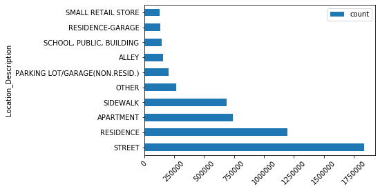
The Location Description field represents areas with the most common crime locations. We will write a function to group our data by location description. This will help us count the number of crimes occurring at each location type.
def groupby_description():
    from datetime import datetime as dt
    # crime data is stored in a feature service and accessed as a DataFrame via the layers object
    df = layers[0]
    # group the dataframe by Location Description field and count the number of crimes for each Location Description.
    out = df.groupBy('Location Description').count()
    # Write the final result to our datastore.
    out.write.format("webgis").save("groupby_location_description" + str(dt.now().microsecond))
run_python_script(code=groupby_description, layers=[crime_lyr])[{'type': 'esriJobMessageTypeInformative',
'description': 'Executing (RunPythonScript): RunPythonScript "def groupby_description():\\n from datetime import datetime as dt\\n # crime data is stored in a feature service and accessed as a DataFrame via the layers object\\n df = layers[0]\\n # group the dataframe by Location Description field and count the number of crimes for each Location Description. \\n out = df.groupBy(\'Location Description\').count()\\n # Write the final result to our datastore.\\n out.write.format("webgis").save("groupby_location_description" + str(dt.now().microsecond))\\n\\ngroupby_description()" https://ndhga01.esri.com/gis/rest/services/DataStoreCatalogs/bigDataFileShares_Chicago_Crime_2001_2020/BigDataCatalogServer/crime "{"defaultAggregationStyles": false, "processSR": {"wkid": 26771}}"'},
{'type': 'esriJobMessageTypeInformative',
'description': 'Start Time: Thu Apr 9 18:21:15 2020'},
{'type': 'esriJobMessageTypeInformative',
'description': 'Using URL based GPRecordSet param: https://ndhga01.esri.com/gis/rest/services/DataStoreCatalogs/bigDataFileShares_Chicago_Crime_2001_2020/BigDataCatalogServer/crime'},
{'type': 'esriJobMessageTypeInformative',
'description': '{"messageCode":"BD_101028","message":"Starting new distributed job with 259 tasks.","params":{"totalTasks":"259"}}'},
{'type': 'esriJobMessageTypeInformative',
'description': '{"messageCode":"BD_101029","message":"0/259 distributed tasks completed.","params":{"completedTasks":"0","totalTasks":"259"}}'},
{'type': 'esriJobMessageTypeInformative',
'description': '{"messageCode":"BD_101029","message":"1/259 distributed tasks completed.","params":{"completedTasks":"1","totalTasks":"259"}}'},
{'type': 'esriJobMessageTypeInformative',
'description': '{"messageCode":"BD_101029","message":"18/259 distributed tasks completed.","params":{"completedTasks":"18","totalTasks":"259"}}'},
{'type': 'esriJobMessageTypeInformative',
'description': '{"messageCode":"BD_101029","message":"41/259 distributed tasks completed.","params":{"completedTasks":"41","totalTasks":"259"}}'},
{'type': 'esriJobMessageTypeInformative',
'description': '{"messageCode":"BD_101029","message":"60/259 distributed tasks completed.","params":{"completedTasks":"60","totalTasks":"259"}}'},
{'type': 'esriJobMessageTypeInformative',
'description': '{"messageCode":"BD_101029","message":"259/259 distributed tasks completed.","params":{"completedTasks":"259","totalTasks":"259"}}'},
{'type': 'esriJobMessageTypeInformative',
'description': '{"messageCode":"BD_101081","message":"Finished writing results:"}'},
{'type': 'esriJobMessageTypeInformative',
'description': '{"messageCode":"BD_101082","message":"* Count of features = 181","params":{"resultCount":"181"}}'},
{'type': 'esriJobMessageTypeInformative',
'description': '{"messageCode":"BD_101083","message":"* Spatial extent = None","params":{"extent":"None"}}'},
{'type': 'esriJobMessageTypeInformative',
'description': '{"messageCode":"BD_101084","message":"* Temporal extent = None","params":{"extent":"None"}}'},
{'type': 'esriJobMessageTypeInformative',
'description': '{"messageCode":"BD_101226","message":"Feature service layer created: https://ndhagsb01.esri.com/gis/rest/services/Hosted/groupby_location_description595817/FeatureServer/0","params":{"serviceUrl":"https://ndhagsb01.esri.com/gis/rest/services/Hosted/groupby_location_description595817/FeatureServer/0"}}'},
{'type': 'esriJobMessageTypeInformative',
'description': 'Succeeded at Thu Apr 9 18:22:03 2020 (Elapsed Time: 48.18 seconds)'}]The result is saved as a feature layer. We can Search for the saved item using the search() method. Providing the search keyword same as the name we used for writing the result will retrieve the layer.
groupby_description = gis.content.search('groupby_location_description')[0]
groupby_description_lyr = groupby_description.tables[0] #retrieve table from the item
groupby_description_df = groupby_description_lyr.query(as_df=True) #read layer as dataframe
groupby_description_df.sort_values(by='count', ascending=False, inplace=True) #sort count field in decreasing order
Location of crime
groupby_description_df[:10].plot(x='Location_Description',
                                 y='count', kind='barh')
plt.xticks(
    rotation=45,
    horizontalalignment='center',
    fontweight='light',
    fontsize='medium',
);
Street is the most frequent location for crime occurrance.
The Primary Type field contains the type for the crime. Let's investigate the most frequent type of crime in the Chicago by writing our own function:
def groupby_texttype():
    from datetime import datetime as dt
    # crime data is stored in a feature service and accessed as a DataFrame via the layers object
    df = layers[0]
    # group the dataframe by TextType field and count the crime incidents for each crime type.
    out = df.groupBy('Primary Type').count()
    # Write the final result to our datastore.
    out.write.format("webgis").save("groupby_type_of_crime" + str(dt.now().microsecond))
run_python_script(code=groupby_texttype, layers=[crime_lyr])[{'type': 'esriJobMessageTypeInformative',
'description': 'Executing (RunPythonScript): RunPythonScript "def groupby_texttype():\\n from datetime import datetime as dt\\n # Calls data is stored in a feature service and accessed as a DataFrame via the layers object\\n df = layers[0]\\n # group the dataframe by TextType field and count the number of calls for each call type. \\n out = df.groupBy(\'Primary Type\').count()\\n # Write the final result to our datastore.\\n out.write.format("webgis").save("groupby_type_of_crime" + str(dt.now().microsecond))\\n\\ngroupby_texttype()" https://ndhga01.esri.com/gis/rest/services/DataStoreCatalogs/bigDataFileShares_Chicago_Crime_2001_2020/BigDataCatalogServer/crime "{"defaultAggregationStyles": false, "processSR": {"wkid": 26771}}"'},
{'type': 'esriJobMessageTypeInformative',
'description': 'Start Time: Thu Apr 9 18:55:46 2020'},
{'type': 'esriJobMessageTypeInformative',
'description': 'Using URL based GPRecordSet param: https://ndhga01.esri.com/gis/rest/services/DataStoreCatalogs/bigDataFileShares_Chicago_Crime_2001_2020/BigDataCatalogServer/crime'},
{'type': 'esriJobMessageTypeInformative',
'description': '{"messageCode":"BD_101028","message":"Starting new distributed job with 259 tasks.","params":{"totalTasks":"259"}}'},
{'type': 'esriJobMessageTypeInformative',
'description': '{"messageCode":"BD_101029","message":"0/259 distributed tasks completed.","params":{"completedTasks":"0","totalTasks":"259"}}'},
{'type': 'esriJobMessageTypeInformative',
'description': '{"messageCode":"BD_101029","message":"1/259 distributed tasks completed.","params":{"completedTasks":"1","totalTasks":"259"}}'},
{'type': 'esriJobMessageTypeInformative',
'description': '{"messageCode":"BD_101029","message":"22/259 distributed tasks completed.","params":{"completedTasks":"22","totalTasks":"259"}}'},
{'type': 'esriJobMessageTypeInformative',
'description': '{"messageCode":"BD_101029","message":"44/259 distributed tasks completed.","params":{"completedTasks":"44","totalTasks":"259"}}'},
{'type': 'esriJobMessageTypeInformative',
'description': '{"messageCode":"BD_101029","message":"259/259 distributed tasks completed.","params":{"completedTasks":"259","totalTasks":"259"}}'},
{'type': 'esriJobMessageTypeInformative',
'description': '{"messageCode":"BD_101081","message":"Finished writing results:"}'},
{'type': 'esriJobMessageTypeInformative',
'description': '{"messageCode":"BD_101082","message":"* Count of features = 35","params":{"resultCount":"35"}}'},
{'type': 'esriJobMessageTypeInformative',
'description': '{"messageCode":"BD_101083","message":"* Spatial extent = None","params":{"extent":"None"}}'},
{'type': 'esriJobMessageTypeInformative',
'description': '{"messageCode":"BD_101084","message":"* Temporal extent = None","params":{"extent":"None"}}'},
{'type': 'esriJobMessageTypeInformative',
'description': '{"messageCode":"BD_101226","message":"Feature service layer created: https://ndhagsb01.esri.com/gis/rest/services/Hosted/groupby_type_of_crime538317/FeatureServer/0","params":{"serviceUrl":"https://ndhagsb01.esri.com/gis/rest/services/Hosted/groupby_type_of_crime538317/FeatureServer/0"}}'},
{'type': 'esriJobMessageTypeInformative',
'description': 'Succeeded at Thu Apr 9 18:56:26 2020 (Elapsed Time: 39.68 seconds)'}]groupby_texttype = gis.content.search('groupby_type_of_crime')[0]groupby_texttypegroupby_texttype_df = groupby_texttype.tables[0].query(as_df=True)groupby_texttype_df.head()| Primary_Type | count | globalid | OBJECTID | |
|---|---|---|---|---|
| 0 | OFFENSE INVOLVING CHILDREN | 48412 | {4120ABC0-FE3A-BBE0-ABC7-B885EEB2D5D2} | 9 |
| 1 | STALKING | 3644 | {52CC61CF-D8DE-D67B-4FC3-C8DD5DB175DE} | 20 |
| 2 | PUBLIC PEACE VIOLATION | 49583 | {4E902E77-D398-72D5-1E3C-EECF4A77B90E} | 26 |
| 3 | OBSCENITY | 650 | {A304388C-A37A-505E-D403-A90F83B04A77} | 34 |
| 4 | ARSON | 11603 | {E65FA2C6-9678-F283-A7B3-E61A40B12674} | 52 |
groupby_texttype_df.sort_values(by='count', ascending=False, inplace=True)Type of crime
groupby_texttype_df.head(10).plot(x='Primary_Type', y='count', kind='barh')
plt.xticks(
    rotation=45,
    horizontalalignment='center',
    fontweight='light',
    fontsize='medium',
);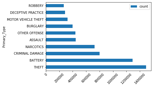
Theft is the most common type of crime in the city of Chicago.
theft = groupby_texttype_df[groupby_texttype_df['Primary_Type'] == 'THEFT']theft| Primary_Type | count | globalid | OBJECTID | |
|---|---|---|---|---|
| 12 | THEFT | 1493302 | {0CBB34E2-58C8-7D0B-01B4-D3E9CE832DC9} | 102 |
def theft_description():
    from datetime import datetime as dt
    # crime data is stored in a feature service and accessed as a DataFrame via the layers object
    df = layers[0]
    df[df['Primary Type'] == 'THEFT']
    out = df.groupBy('Location Description').count()
    # Write the final result to our datastore.
    out.write.format("webgis").save("theft_description" + str(dt.now().microsecond))
run_python_script(code=theft_description, layers=[crime_lyr])[{'type': 'esriJobMessageTypeInformative',
'description': 'Executing (RunPythonScript): RunPythonScript "def theft_description():\\n from datetime import datetime as dt\\n # Calls data is stored in a feature service and accessed as a DataFrame via the layers object\\n df = layers[0]\\n df[df[\'Primary Type\'] == \'THEFT\']\\n out = df.groupBy(\'Location Description\').count()\\n # Write the final result to our datastore.\\n out.write.format("webgis").save("theft_description" + str(dt.now().microsecond))\\n\\ntheft_description()" https://ndhga01.esri.com/gis/rest/services/DataStoreCatalogs/bigDataFileShares_Chicago_Crime_2001_2020/BigDataCatalogServer/crime "{"defaultAggregationStyles": false, "processSR": {"wkid": 26771}}"'},
{'type': 'esriJobMessageTypeInformative',
'description': 'Start Time: Thu Apr 9 18:56:30 2020'},
{'type': 'esriJobMessageTypeInformative',
'description': 'Using URL based GPRecordSet param: https://ndhga01.esri.com/gis/rest/services/DataStoreCatalogs/bigDataFileShares_Chicago_Crime_2001_2020/BigDataCatalogServer/crime'},
{'type': 'esriJobMessageTypeInformative',
'description': '{"messageCode":"BD_101028","message":"Starting new distributed job with 259 tasks.","params":{"totalTasks":"259"}}'},
{'type': 'esriJobMessageTypeInformative',
'description': '{"messageCode":"BD_101029","message":"0/259 distributed tasks completed.","params":{"completedTasks":"0","totalTasks":"259"}}'},
{'type': 'esriJobMessageTypeInformative',
'description': '{"messageCode":"BD_101029","message":"1/259 distributed tasks completed.","params":{"completedTasks":"1","totalTasks":"259"}}'},
{'type': 'esriJobMessageTypeInformative',
'description': '{"messageCode":"BD_101029","message":"24/259 distributed tasks completed.","params":{"completedTasks":"24","totalTasks":"259"}}'},
{'type': 'esriJobMessageTypeInformative',
'description': '{"messageCode":"BD_101029","message":"45/259 distributed tasks completed.","params":{"completedTasks":"45","totalTasks":"259"}}'},
{'type': 'esriJobMessageTypeInformative',
'description': '{"messageCode":"BD_101029","message":"101/259 distributed tasks completed.","params":{"completedTasks":"101","totalTasks":"259"}}'},
{'type': 'esriJobMessageTypeInformative',
'description': '{"messageCode":"BD_101029","message":"259/259 distributed tasks completed.","params":{"completedTasks":"259","totalTasks":"259"}}'},
{'type': 'esriJobMessageTypeInformative',
'description': '{"messageCode":"BD_101081","message":"Finished writing results:"}'},
{'type': 'esriJobMessageTypeInformative',
'description': '{"messageCode":"BD_101082","message":"* Count of features = 181","params":{"resultCount":"181"}}'},
{'type': 'esriJobMessageTypeInformative',
'description': '{"messageCode":"BD_101083","message":"* Spatial extent = None","params":{"extent":"None"}}'},
{'type': 'esriJobMessageTypeInformative',
'description': '{"messageCode":"BD_101084","message":"* Temporal extent = None","params":{"extent":"None"}}'},
{'type': 'esriJobMessageTypeInformative',
'description': '{"messageCode":"BD_101226","message":"Feature service layer created: https://ndhagsb01.esri.com/gis/rest/services/Hosted/theft_description406470/FeatureServer/0","params":{"serviceUrl":"https://ndhagsb01.esri.com/gis/rest/services/Hosted/theft_description406470/FeatureServer/0"}}'},
{'type': 'esriJobMessageTypeInformative',
'description': 'Succeeded at Thu Apr 9 18:57:11 2020 (Elapsed Time: 41.21 seconds)'}]theft_description = gis.content.search('theft_description')[0]theft_description_df = theft_description.tables[0].query(as_df=True)theft_description_df.sort_values(by='count', ascending=False, inplace=True)Location of theft
theft_description_df[:10].plot(x='Location_Description', y='count', kind='barh')
plt.xticks(
    rotation=45,
    horizontalalignment='center',
    fontweight='light',
    fontsize='medium',
);
This plot shows the relation between crime type and crime location. It indicates that most of the theft activities occur on streets.
def grpby_type_blkgrp():
    from datetime import datetime as dt
    # Load the big data file share layer into a DataFrame
    df = layers[0]
    out = df.groupBy('Primary Type', 'Block').count()
    out.write.format("webgis").save("grpby_type_blkgrp" + str(dt.now().microsecond))
run_python_script(code=grpby_type_blkgrp, layers=[crime_lyr])[{'type': 'esriJobMessageTypeInformative',
'description': 'Executing (RunPythonScript): RunPythonScript "def grpby_type_blkgrp():\\n from datetime import datetime as dt\\n # Load the big data file share layer into a DataFrame\\n df = layers[0]\\n out = df.groupBy(\'Primary Type\', \'Block\').count()\\n out.write.format("webgis").save("grpby_type_blkgrp" + str(dt.now().microsecond))\\n\\ngrpby_type_blkgrp()" https://ndhga01.esri.com/gis/rest/services/DataStoreCatalogs/bigDataFileShares_Chicago_Crime_2001_2020/BigDataCatalogServer/crime "{"defaultAggregationStyles": false, "processSR": {"wkid": 26771}}"'},
{'type': 'esriJobMessageTypeInformative',
'description': 'Start Time: Thu Apr 9 18:57:14 2020'},
{'type': 'esriJobMessageTypeInformative',
'description': 'Using URL based GPRecordSet param: https://ndhga01.esri.com/gis/rest/services/DataStoreCatalogs/bigDataFileShares_Chicago_Crime_2001_2020/BigDataCatalogServer/crime'},
{'type': 'esriJobMessageTypeInformative',
'description': '{"messageCode":"BD_101028","message":"Starting new distributed job with 259 tasks.","params":{"totalTasks":"259"}}'},
{'type': 'esriJobMessageTypeInformative',
'description': '{"messageCode":"BD_101029","message":"0/259 distributed tasks completed.","params":{"completedTasks":"0","totalTasks":"259"}}'},
{'type': 'esriJobMessageTypeInformative',
'description': '{"messageCode":"BD_101029","message":"1/259 distributed tasks completed.","params":{"completedTasks":"1","totalTasks":"259"}}'},
{'type': 'esriJobMessageTypeInformative',
'description': '{"messageCode":"BD_101029","message":"25/259 distributed tasks completed.","params":{"completedTasks":"25","totalTasks":"259"}}'},
{'type': 'esriJobMessageTypeInformative',
'description': '{"messageCode":"BD_101029","message":"46/259 distributed tasks completed.","params":{"completedTasks":"46","totalTasks":"259"}}'},
{'type': 'esriJobMessageTypeInformative',
'description': '{"messageCode":"BD_101029","message":"60/259 distributed tasks completed.","params":{"completedTasks":"60","totalTasks":"259"}}'},
{'type': 'esriJobMessageTypeInformative',
'description': '{"messageCode":"BD_101029","message":"118/259 distributed tasks completed.","params":{"completedTasks":"118","totalTasks":"259"}}'},
{'type': 'esriJobMessageTypeInformative',
'description': '{"messageCode":"BD_101029","message":"163/259 distributed tasks completed.","params":{"completedTasks":"163","totalTasks":"259"}}'},
{'type': 'esriJobMessageTypeInformative',
'description': '{"messageCode":"BD_101029","message":"206/259 distributed tasks completed.","params":{"completedTasks":"206","totalTasks":"259"}}'},
{'type': 'esriJobMessageTypeInformative',
'description': '{"messageCode":"BD_101029","message":"245/259 distributed tasks completed.","params":{"completedTasks":"245","totalTasks":"259"}}'},
{'type': 'esriJobMessageTypeInformative',
'description': '{"messageCode":"BD_101029","message":"259/259 distributed tasks completed.","params":{"completedTasks":"259","totalTasks":"259"}}'},
{'type': 'esriJobMessageTypeInformative',
'description': '{"messageCode":"BD_101081","message":"Finished writing results:"}'},
{'type': 'esriJobMessageTypeInformative',
'description': '{"messageCode":"BD_101082","message":"* Count of features = 571108","params":{"resultCount":"571108"}}'},
{'type': 'esriJobMessageTypeInformative',
'description': '{"messageCode":"BD_101083","message":"* Spatial extent = None","params":{"extent":"None"}}'},
{'type': 'esriJobMessageTypeInformative',
'description': '{"messageCode":"BD_101084","message":"* Temporal extent = None","params":{"extent":"None"}}'},
{'type': 'esriJobMessageTypeInformative',
'description': '{"messageCode":"BD_101226","message":"Feature service layer created: https://ndhagsb01.esri.com/gis/rest/services/Hosted/grpby_type_blkgrp322476/FeatureServer/0","params":{"serviceUrl":"https://ndhagsb01.esri.com/gis/rest/services/Hosted/grpby_type_blkgrp322476/FeatureServer/0"}}'},
{'type': 'esriJobMessageTypeInformative',
'description': 'Succeeded at Thu Apr 9 18:58:17 2020 (Elapsed Time: 1 minutes 3 seconds)'}]grpby_cat_blk = gis.content.search('grpby_type_blkgrp')[0]grpby_cat_blkgrpby_cat_blk_df = grpby_cat_blk.tables[0].query(as_df=True)grpby_cat_blk_df.head()| Block | OBJECTID | Primary_Type | count | globalid | |
|---|---|---|---|---|---|
| 0 | 096XX S MICHIGAN AV | 1 | BATTERY | 34 | {AC1470E0-614D-BB2A-901E-034720D62910} |
| 1 | 070XX S LAFAYETTE ST | 2 | ASSAULT | 1 | {5876F9DE-F728-22A9-270C-710E48FA17FB} |
| 2 | 061XX S COTTAGE GROVE | 3 | CRIMINAL TRESPASS | 75 | {3D7FC5D0-F670-53B9-7135-5DB84B1048E4} |
| 3 | 014XX W MONTROSE AV | 4 | OTHER OFFENSE | 1 | {478D77DC-DAFA-C59D-08B0-29911B4F50FD} |
| 4 | 055XX N LAKE SHORE DR | 5 | OTHER OFFENSE | 1 | {69281C9B-5158-8A73-7AEF-1EB4102276C2} |
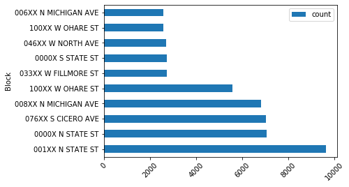
Count of crime incidents by block group
grpby_cat_blk_df.sort_values(by='count', ascending=False, inplace=True)grpby_cat_blk_df.head(10).plot(x='Block', y='count', kind='barh')
plt.xticks(
rotation=45,
horizontalalignment='center',
fontweight='light',
fontsize='medium',
);
Get crime types for a particular block group
blk_addr_high = grpby_cat_blk_df[grpby_cat_blk_df['Block'] == '001XX N STATE ST']blk_addr_high.Primary_Type.sort_values(ascending=False).head()143115 WEAPONS VIOLATION 766 THEFT 122685 STALKING 94954 SEX OFFENSE 28868 ROBBERY Name: Primary_Type, dtype: object
def crime_by_datetime():
    from datetime import datetime as dt
    # Load the big data file share layer into a DataFrame
    from pyspark.sql import functions as F
    df = layers[0]
    out = df.withColumn('datetime', F.unix_timestamp('Date', 'dd/MM/yyyy hh:mm:ss a').cast('timestamp'))
    out.write.format("webgis").save("crime_by_datetime" + str(dt.now().microsecond))
run_python_script(code=crime_by_datetime, layers=[crime_lyr])[{'type': 'esriJobMessageTypeInformative',
'description': 'Executing (RunPythonScript): RunPythonScript "def crime_by_datetime():\\n from datetime import datetime as dt\\n # Load the big data file share layer into a DataFrame\\n from pyspark.sql import functions as F\\n df = layers[0]\\n out = df.withColumn(\'datetime\', F.unix_timestamp(\'Date\', \'dd/MM/yyyy hh:mm:ss a\').cast(\'timestamp\'))\\n out.write.format("webgis").save("crime_by_datetime" + str(dt.now().microsecond))\\n\\ncrime_by_datetime()" https://ndhga01.esri.com/gis/rest/services/DataStoreCatalogs/bigDataFileShares_Chicago_Crime_2001_2020/BigDataCatalogServer/crime "{"defaultAggregationStyles": false, "processSR": {"wkid": 26771}}"'},
{'type': 'esriJobMessageTypeInformative',
'description': 'Start Time: Thu Apr 9 19:39:44 2020'},
{'type': 'esriJobMessageTypeInformative',
'description': 'Using URL based GPRecordSet param: https://ndhga01.esri.com/gis/rest/services/DataStoreCatalogs/bigDataFileShares_Chicago_Crime_2001_2020/BigDataCatalogServer/crime'},
{'type': 'esriJobMessageTypeInformative',
'description': '{"messageCode":"BD_101028","message":"Starting new distributed job with 59 tasks.","params":{"totalTasks":"59"}}'},
{'type': 'esriJobMessageTypeInformative',
'description': '{"messageCode":"BD_101029","message":"0/59 distributed tasks completed.","params":{"completedTasks":"0","totalTasks":"59"}}'},
{'type': 'esriJobMessageTypeInformative',
'description': '{"messageCode":"BD_101029","message":"1/59 distributed tasks completed.","params":{"completedTasks":"1","totalTasks":"59"}}'},
{'type': 'esriJobMessageTypeInformative',
'description': '{"messageCode":"BD_101029","message":"5/59 distributed tasks completed.","params":{"completedTasks":"5","totalTasks":"59"}}'},
{'type': 'esriJobMessageTypeInformative',
'description': '{"messageCode":"BD_101029","message":"6/59 distributed tasks completed.","params":{"completedTasks":"6","totalTasks":"59"}}'},
{'type': 'esriJobMessageTypeInformative',
'description': '{"messageCode":"BD_101029","message":"13/59 distributed tasks completed.","params":{"completedTasks":"13","totalTasks":"59"}}'},
{'type': 'esriJobMessageTypeInformative',
'description': '{"messageCode":"BD_101029","message":"19/59 distributed tasks completed.","params":{"completedTasks":"19","totalTasks":"59"}}'},
{'type': 'esriJobMessageTypeInformative',
'description': '{"messageCode":"BD_101029","message":"24/59 distributed tasks completed.","params":{"completedTasks":"24","totalTasks":"59"}}'},
{'type': 'esriJobMessageTypeInformative',
'description': '{"messageCode":"BD_101029","message":"25/59 distributed tasks completed.","params":{"completedTasks":"25","totalTasks":"59"}}'},
{'type': 'esriJobMessageTypeInformative',
'description': '{"messageCode":"BD_101029","message":"26/59 distributed tasks completed.","params":{"completedTasks":"26","totalTasks":"59"}}'},
{'type': 'esriJobMessageTypeInformative',
'description': '{"messageCode":"BD_101029","message":"29/59 distributed tasks completed.","params":{"completedTasks":"29","totalTasks":"59"}}'},
{'type': 'esriJobMessageTypeInformative',
'description': '{"messageCode":"BD_101029","message":"33/59 distributed tasks completed.","params":{"completedTasks":"33","totalTasks":"59"}}'},
{'type': 'esriJobMessageTypeInformative',
'description': '{"messageCode":"BD_101029","message":"37/59 distributed tasks completed.","params":{"completedTasks":"37","totalTasks":"59"}}'},
{'type': 'esriJobMessageTypeInformative',
'description': '{"messageCode":"BD_101029","message":"40/59 distributed tasks completed.","params":{"completedTasks":"40","totalTasks":"59"}}'},
{'type': 'esriJobMessageTypeInformative',
'description': '{"messageCode":"BD_101029","message":"43/59 distributed tasks completed.","params":{"completedTasks":"43","totalTasks":"59"}}'},
{'type': 'esriJobMessageTypeInformative',
'description': '{"messageCode":"BD_101029","message":"46/59 distributed tasks completed.","params":{"completedTasks":"46","totalTasks":"59"}}'},
{'type': 'esriJobMessageTypeInformative',
'description': '{"messageCode":"BD_101029","message":"59/59 distributed tasks completed.","params":{"completedTasks":"59","totalTasks":"59"}}'},
{'type': 'esriJobMessageTypeInformative',
'description': '{"messageCode":"BD_101081","message":"Finished writing results:"}'},
{'type': 'esriJobMessageTypeInformative',
'description': '{"messageCode":"BD_101082","message":"* Count of features = 7061128","params":{"resultCount":"7061128"}}'},
{'type': 'esriJobMessageTypeInformative',
'description': '{"messageCode":"BD_101083","message":"* Spatial extent = {\\"xmin\\":-91.686565684,\\"ymin\\":36.619446395,\\"xmax\\":-87.524529378,\\"ymax\\":42.022910333}","params":{"extent":"{\\"xmin\\":-91.686565684,\\"ymin\\":36.619446395,\\"xmax\\":-87.524529378,\\"ymax\\":42.022910333}"}}'},
{'type': 'esriJobMessageTypeInformative',
'description': '{"messageCode":"BD_101084","message":"* Temporal extent = Interval(MutableInstant(2001-01-01 00:00:00.000),MutableInstant(2020-01-26 23:40:00.000))","params":{"extent":"Interval(MutableInstant(2001-01-01 00:00:00.000),MutableInstant(2020-01-26 23:40:00.000))"}}'},
{'type': 'esriJobMessageTypeInformative',
'description': '{"messageCode":"BD_101226","message":"Feature service layer created: https://ndhagsb01.esri.com/gis/rest/services/Hosted/crime_by_datetime650380/FeatureServer/0","params":{"serviceUrl":"https://ndhagsb01.esri.com/gis/rest/services/Hosted/crime_by_datetime650380/FeatureServer/0"}}'},
{'type': 'esriJobMessageTypeInformative',
'description': 'Succeeded at Thu Apr 9 19:42:31 2020 (Elapsed Time: 2 minutes 46 seconds)'}]calls_with_datetime = gis.content.search('crime_by_datetime')[0]calls_with_datetime_lyr = calls_with_datetime.layers[0]def crime_with_added_date_time_cols():
from datetime import datetime as dt
# Load the big data file share layer into a DataFrame
from pyspark.sql.functions import year, month, hour
df = layers[0]
df = df.withColumn('month', month(df['datetime']))
out = df.withColumn('hour', hour(df['datetime']))
out.write.format("webgis").save("crime_with_added_date_time_cols" + str(dt.now().microsecond))run_python_script(code=crime_with_added_date_time_cols, layers=[calls_with_datetime_lyr])[{'type': 'esriJobMessageTypeInformative',
'description': 'Executing (RunPythonScript): RunPythonScript "def crime_with_added_date_time_cols():\\n from datetime import datetime as dt\\n # Load the big data file share layer into a DataFrame\\n from pyspark.sql.functions import year, month, hour\\n df = layers[0]\\n df = df.withColumn(\'month\', month(df[\'datetime\']))\\n out = df.withColumn(\'hour\', hour(df[\'datetime\']))\\n out.write.format("webgis").save("crime_with_added_date_time_cols" + str(dt.now().microsecond))\\n\\ncrime_with_added_date_time_cols()" https://ndhagsb01.esri.com/gis/rest/services/Hosted/crime_by_datetime650380/FeatureServer/0 "{"defaultAggregationStyles": false, "processSR": {"wkid": 26771}}"'},
{'type': 'esriJobMessageTypeInformative',
'description': 'Start Time: Thu Apr 9 19:42:34 2020'},
{'type': 'esriJobMessageTypeInformative',
'description': 'Using URL based GPRecordSet param: https://ndhagsb01.esri.com/gis/rest/services/Hosted/crime_by_datetime650380/FeatureServer/0'},
{'type': 'esriJobMessageTypeInformative',
'description': '{"messageCode":"BD_101028","message":"Starting new distributed job with 66 tasks.","params":{"totalTasks":"66"}}'},
{'type': 'esriJobMessageTypeInformative',
'description': '{"messageCode":"BD_101029","message":"0/66 distributed tasks completed.","params":{"completedTasks":"0","totalTasks":"66"}}'},
{'type': 'esriJobMessageTypeInformative',
'description': '{"messageCode":"BD_101029","message":"1/66 distributed tasks completed.","params":{"completedTasks":"1","totalTasks":"66"}}'},
{'type': 'esriJobMessageTypeInformative',
'description': '{"messageCode":"BD_101029","message":"3/66 distributed tasks completed.","params":{"completedTasks":"3","totalTasks":"66"}}'},
{'type': 'esriJobMessageTypeInformative',
'description': '{"messageCode":"BD_101029","message":"10/66 distributed tasks completed.","params":{"completedTasks":"10","totalTasks":"66"}}'},
{'type': 'esriJobMessageTypeInformative',
'description': '{"messageCode":"BD_101029","message":"15/66 distributed tasks completed.","params":{"completedTasks":"15","totalTasks":"66"}}'},
{'type': 'esriJobMessageTypeInformative',
'description': '{"messageCode":"BD_101029","message":"19/66 distributed tasks completed.","params":{"completedTasks":"19","totalTasks":"66"}}'},
{'type': 'esriJobMessageTypeInformative',
'description': '{"messageCode":"BD_101029","message":"22/66 distributed tasks completed.","params":{"completedTasks":"22","totalTasks":"66"}}'},
{'type': 'esriJobMessageTypeInformative',
'description': '{"messageCode":"BD_101029","message":"24/66 distributed tasks completed.","params":{"completedTasks":"24","totalTasks":"66"}}'},
{'type': 'esriJobMessageTypeInformative',
'description': '{"messageCode":"BD_101029","message":"29/66 distributed tasks completed.","params":{"completedTasks":"29","totalTasks":"66"}}'},
{'type': 'esriJobMessageTypeInformative',
'description': '{"messageCode":"BD_101029","message":"32/66 distributed tasks completed.","params":{"completedTasks":"32","totalTasks":"66"}}'},
{'type': 'esriJobMessageTypeInformative',
'description': '{"messageCode":"BD_101029","message":"36/66 distributed tasks completed.","params":{"completedTasks":"36","totalTasks":"66"}}'},
{'type': 'esriJobMessageTypeInformative',
'description': '{"messageCode":"BD_101029","message":"37/66 distributed tasks completed.","params":{"completedTasks":"37","totalTasks":"66"}}'},
{'type': 'esriJobMessageTypeInformative',
'description': '{"messageCode":"BD_101029","message":"38/66 distributed tasks completed.","params":{"completedTasks":"38","totalTasks":"66"}}'},
{'type': 'esriJobMessageTypeInformative',
'description': '{"messageCode":"BD_101029","message":"42/66 distributed tasks completed.","params":{"completedTasks":"42","totalTasks":"66"}}'},
{'type': 'esriJobMessageTypeInformative',
'description': '{"messageCode":"BD_101029","message":"43/66 distributed tasks completed.","params":{"completedTasks":"43","totalTasks":"66"}}'},
{'type': 'esriJobMessageTypeInformative',
'description': '{"messageCode":"BD_101029","message":"46/66 distributed tasks completed.","params":{"completedTasks":"46","totalTasks":"66"}}'},
{'type': 'esriJobMessageTypeInformative',
'description': '{"messageCode":"BD_101029","message":"51/66 distributed tasks completed.","params":{"completedTasks":"51","totalTasks":"66"}}'},
{'type': 'esriJobMessageTypeInformative',
'description': '{"messageCode":"BD_101029","message":"55/66 distributed tasks completed.","params":{"completedTasks":"55","totalTasks":"66"}}'},
{'type': 'esriJobMessageTypeInformative',
'description': '{"messageCode":"BD_101029","message":"56/66 distributed tasks completed.","params":{"completedTasks":"56","totalTasks":"66"}}'},
{'type': 'esriJobMessageTypeInformative',
'description': '{"messageCode":"BD_101029","message":"60/66 distributed tasks completed.","params":{"completedTasks":"60","totalTasks":"66"}}'},
{'type': 'esriJobMessageTypeInformative',
'description': '{"messageCode":"BD_101029","message":"66/66 distributed tasks completed.","params":{"completedTasks":"66","totalTasks":"66"}}'},
{'type': 'esriJobMessageTypeInformative',
'description': '{"messageCode":"BD_101081","message":"Finished writing results:"}'},
{'type': 'esriJobMessageTypeInformative',
'description': '{"messageCode":"BD_101082","message":"* Count of features = 7061128","params":{"resultCount":"7061128"}}'},
{'type': 'esriJobMessageTypeInformative',
'description': '{"messageCode":"BD_101083","message":"* Spatial extent = {\\"xmin\\":-91.686565684,\\"ymin\\":36.619446395,\\"xmax\\":-87.524529378,\\"ymax\\":42.022910333}","params":{"extent":"{\\"xmin\\":-91.686565684,\\"ymin\\":36.619446395,\\"xmax\\":-87.524529378,\\"ymax\\":42.022910333}"}}'},
{'type': 'esriJobMessageTypeInformative',
'description': '{"messageCode":"BD_101084","message":"* Temporal extent = Interval(MutableInstant(2001-01-01 00:00:00.000),MutableInstant(2020-01-26 23:40:00.000))","params":{"extent":"Interval(MutableInstant(2001-01-01 00:00:00.000),MutableInstant(2020-01-26 23:40:00.000))"}}'},
{'type': 'esriJobMessageTypeInformative',
'description': '{"messageCode":"BD_101226","message":"Feature service layer created: https://ndhagsb01.esri.com/gis/rest/services/Hosted/crime_with_added_date_time_cols749239/FeatureServer/0","params":{"serviceUrl":"https://ndhagsb01.esri.com/gis/rest/services/Hosted/crime_with_added_date_time_cols749239/FeatureServer/0"}}'},
{'type': 'esriJobMessageTypeInformative',
'description': 'Succeeded at Thu Apr 9 19:47:06 2020 (Elapsed Time: 4 minutes 32 seconds)'}]date_time_added_item = gis.content.search('crime_with_added_date_time_cols')date_time_added_lyr = date_time_added_item[0].layers[0]def grp_crime_by_hour():
from datetime import datetime as dt
# Load the big data file share layer into a DataFrame
df = layers[0]
out = df.groupBy('hour').count()
out.write.format("webgis").save("grp_crime_by_hour" + str(dt.now().microsecond))run_python_script(code=grp_crime_by_hour, layers=[date_time_added_lyr])[{'type': 'esriJobMessageTypeInformative',
'description': 'Executing (RunPythonScript): RunPythonScript "def grp_crime_by_hour():\\n from datetime import datetime as dt\\n # Load the big data file share layer into a DataFrame\\n df = layers[0]\\n out = df.groupBy(\'hour\').count()\\n out.write.format("webgis").save("grp_crime_by_hour" + str(dt.now().microsecond))\\n\\ngrp_crime_by_hour()" https://ndhagsb01.esri.com/gis/rest/services/Hosted/crime_with_added_date_time_cols749239/FeatureServer/0 "{"defaultAggregationStyles": false, "processSR": {"wkid": 26771}}"'},
{'type': 'esriJobMessageTypeInformative',
'description': 'Start Time: Thu Apr 9 19:47:09 2020'},
{'type': 'esriJobMessageTypeInformative',
'description': 'Using URL based GPRecordSet param: https://ndhagsb01.esri.com/gis/rest/services/Hosted/crime_with_added_date_time_cols749239/FeatureServer/0'},
{'type': 'esriJobMessageTypeInformative',
'description': '{"messageCode":"BD_101028","message":"Starting new distributed job with 266 tasks.","params":{"totalTasks":"266"}}'},
{'type': 'esriJobMessageTypeInformative',
'description': '{"messageCode":"BD_101029","message":"0/266 distributed tasks completed.","params":{"completedTasks":"0","totalTasks":"266"}}'},
{'type': 'esriJobMessageTypeInformative',
'description': '{"messageCode":"BD_101029","message":"1/266 distributed tasks completed.","params":{"completedTasks":"1","totalTasks":"266"}}'},
{'type': 'esriJobMessageTypeInformative',
'description': '{"messageCode":"BD_101029","message":"7/266 distributed tasks completed.","params":{"completedTasks":"7","totalTasks":"266"}}'},
{'type': 'esriJobMessageTypeInformative',
'description': '{"messageCode":"BD_101029","message":"11/266 distributed tasks completed.","params":{"completedTasks":"11","totalTasks":"266"}}'},
{'type': 'esriJobMessageTypeInformative',
'description': '{"messageCode":"BD_101029","message":"19/266 distributed tasks completed.","params":{"completedTasks":"19","totalTasks":"266"}}'},
{'type': 'esriJobMessageTypeInformative',
'description': '{"messageCode":"BD_101029","message":"25/266 distributed tasks completed.","params":{"completedTasks":"25","totalTasks":"266"}}'},
{'type': 'esriJobMessageTypeInformative',
'description': '{"messageCode":"BD_101029","message":"27/266 distributed tasks completed.","params":{"completedTasks":"27","totalTasks":"266"}}'},
{'type': 'esriJobMessageTypeInformative',
'description': '{"messageCode":"BD_101029","message":"32/266 distributed tasks completed.","params":{"completedTasks":"32","totalTasks":"266"}}'},
{'type': 'esriJobMessageTypeInformative',
'description': '{"messageCode":"BD_101029","message":"36/266 distributed tasks completed.","params":{"completedTasks":"36","totalTasks":"266"}}'},
{'type': 'esriJobMessageTypeInformative',
'description': '{"messageCode":"BD_101029","message":"41/266 distributed tasks completed.","params":{"completedTasks":"41","totalTasks":"266"}}'},
{'type': 'esriJobMessageTypeInformative',
'description': '{"messageCode":"BD_101029","message":"45/266 distributed tasks completed.","params":{"completedTasks":"45","totalTasks":"266"}}'},
{'type': 'esriJobMessageTypeInformative',
'description': '{"messageCode":"BD_101029","message":"52/266 distributed tasks completed.","params":{"completedTasks":"52","totalTasks":"266"}}'},
{'type': 'esriJobMessageTypeInformative',
'description': '{"messageCode":"BD_101029","message":"58/266 distributed tasks completed.","params":{"completedTasks":"58","totalTasks":"266"}}'},
{'type': 'esriJobMessageTypeInformative',
'description': '{"messageCode":"BD_101029","message":"62/266 distributed tasks completed.","params":{"completedTasks":"62","totalTasks":"266"}}'},
{'type': 'esriJobMessageTypeInformative',
'description': '{"messageCode":"BD_101029","message":"266/266 distributed tasks completed.","params":{"completedTasks":"266","totalTasks":"266"}}'},
{'type': 'esriJobMessageTypeInformative',
'description': '{"messageCode":"BD_101081","message":"Finished writing results:"}'},
{'type': 'esriJobMessageTypeInformative',
'description': '{"messageCode":"BD_101082","message":"* Count of features = 25","params":{"resultCount":"25"}}'},
{'type': 'esriJobMessageTypeInformative',
'description': '{"messageCode":"BD_101083","message":"* Spatial extent = None","params":{"extent":"None"}}'},
{'type': 'esriJobMessageTypeInformative',
'description': '{"messageCode":"BD_101084","message":"* Temporal extent = None","params":{"extent":"None"}}'},
{'type': 'esriJobMessageTypeInformative',
'description': '{"messageCode":"BD_101226","message":"Feature service layer created: https://ndhagsb01.esri.com/gis/rest/services/Hosted/grp_crime_by_hour391644/FeatureServer/0","params":{"serviceUrl":"https://ndhagsb01.esri.com/gis/rest/services/Hosted/grp_crime_by_hour391644/FeatureServer/0"}}'},
{'type': 'esriJobMessageTypeInformative',
'description': 'Succeeded at Thu Apr 9 19:49:15 2020 (Elapsed Time: 2 minutes 5 seconds)'}]hour = gis.content.search('grp_crime_by_hour')[0]grp_hour = hour.tables[0]df_hour = grp_hour.query(as_df=True)Crime distribution by the hour
(df_hour
 .dropna()
 .sort_values(by='hour')
 .astype({'hour' : int})
 .plot(x='hour', y='count', kind='bar'))
plt.xticks(
    rotation=45,
    horizontalalignment='center',
    fontweight='light',
    fontsize='medium',
);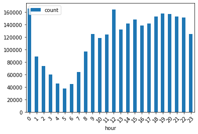
This graph shows that the crime activities are more common at the peak hours 12 A.M. and 12 P.M.
Big data machine learning using pyspark.ml
Find the optimal number of clusters
The average silhouette approach measures the quality of a clustering. That is, it determines how well each object lies within its cluster. A high average silhouette width indicates a good clustering. To learn more about silhouette analysis, click here.
def optimal_k():
    import time
    import numpy as np
    import pandas as pd
    from pyspark.ml.feature import VectorAssembler
    from pyspark.ml.clustering import KMeans
    from datetime import datetime as dt
    from pyspark.ml.evaluation import ClusteringEvaluator
    from pyspark.sql.context import SQLContext
    from pyspark.sql.types import StructType, StructField, DoubleType, IntegerType, FloatType

    silh_lst = []
    k_lst = np.arange(3, 70)

    crime_locations = layers[0]
    assembler = VectorAssembler(inputCols=["X Coordinate", "Y Coordinate"], outputCol="features")
    crime_locations = assembler.setHandleInvalid("skip").transform(crime_locations)

    for k in k_lst:
        silh_val = []
        for run in np.arange(1, 3):
            # Trains a k-means model.
            kmeans = KMeans().setK(int(k)).setSeed(int(np.random.randint(100, size=1)))
            model = kmeans.fit(crime_locations.select("features"))

            # Make predictions
            predictions = model.transform(crime_locations)

            # Evaluate clustering by computing Silhouette score
            evaluator = ClusteringEvaluator()
            silhouette = evaluator.evaluate(predictions)
            silh_val.append(silhouette)

        silh_array=np.asanyarray(silh_val)
        silh_lst.append(silh_array.mean())

    silhouette = pd.DataFrame(list(zip(k_lst,silh_lst)),columns = ['k', 'silhouette'])
    schema = StructType([StructField('k',IntegerType(),True), StructField('silhouette',FloatType(),True)])
    out = SQLContext(sparkContext=spark.sparkContext, sparkSession=spark).createDataFrame(silhouette, schema)
    # Write the result DataFrame to the relational data store
    out.write.format("webgis").option("dataStore","relational").save("optimalKmeans" + str(dt.now().microsecond))
run_python_script(code=optimal_k, layers=[crime_lyr])optimal_k = gis.content.search('optimalKmeans')[0]optimal_k_tbl = optimal_k.tables[0]k_df = optimal_k_tbl.query().sdfk_df.sort_values(by='silhouette', ascending=False)| objectid | k | silhouette | |
|---|---|---|---|
| 54 | 58 | 15 | 0.556612 |
| 22 | 23 | 19 | 0.556012 |
| 2 | 3 | 9 | 0.555995 |
| 39 | 40 | 14 | 0.552853 |
| 38 | 39 | 11 | 0.551726 |
| ... | ... | ... | ... |
| 24 | 25 | 25 | 0.527496 |
| 19 | 20 | 7 | 0.527266 |
| 26 | 27 | 34 | 0.525585 |
| 37 | 38 | 8 | 0.507064 |
| 36 | 37 | 5 | 0.492071 |
67 rows × 3 columns
num_clusters = k_df.sort_values(by='silhouette', ascending=False).loc[0]['k']
num_clusters
15
K-Means Clustering
def cluster_crimes():

    from pyspark.ml.feature import VectorAssembler
    from pyspark.ml.clustering import KMeans
    from datetime import datetime as dt
    # Crime data is stored in a feature service and accessed as a DataFrame via the layers object
    crime_locations = layers[0]

    # Combine the x and y columns in the DataFrame into a single column called "features"
    assembler = VectorAssembler(inputCols=["X Coordinate", "Y Coordinate"], outputCol="features")
    crime_locations = assembler.setHandleInvalid("skip").transform(crime_locations)

    # Fit a k-means model with 15 clusters using the "features" column of the crime locations
    kmeans = KMeans(k=15)
    model = kmeans.fit(crime_locations.select("features"))

    cost = model.computeCost(crime_locations)
    # Add the cluster labels from the k-means model to the original DataFrame
    crime_locations_clusters = model.transform(crime_locations)
    # Write the result DataFrame to the relational data store
    crime_locations_clusters.write.format("webgis").save("Crime_Clusters_KMeans" + str(dt.now().microsecond))
run_python_script(code=cluster_crimes, layers=[crime_lyr]){"messageCode":"BD_101231","message":"The following fields are not supported and will be dropped: features","params":{"fields":"features"}}
[{'type': 'esriJobMessageTypeInformative',
  'description': 'Executing (RunPythonScript): RunPythonScript "def cluster_crimes():\\n    \\n    from pyspark.ml.feature import VectorAssembler\\n    from pyspark.ml.clustering import KMeans\\n    from datetime import datetime as dt\\n    # Crime data is stored in a feature service and accessed as a DataFrame via the layers object\\n    crime_locations = layers[0]\\n    \\n    # Combine the x and y columns in the DataFrame into a single column called "features"\\n    assembler = VectorAssembler(inputCols=["X Coordinate", "Y Coordinate"], outputCol="features")\\n    crime_locations = assembler.setHandleInvalid("skip").transform(crime_locations)\\n\\n    # Fit a k-means model with 50 clusters using the "features" column of the crime locations\\n    kmeans = KMeans(k=15)\\n    model = kmeans.fit(crime_locations.select("features"))\\n    \\n    cost = model.computeCost(crime_locations)\\n    print(\'cost\', cost)\\n    # Add the cluster labels from the k-means model to the original DataFrame\\n    crime_locations_clusters = model.transform(crime_locations)\\n    # Write the result DataFrame to the relational data store\\n    crime_locations_clusters.write.format("webgis").save("Crime_Clusters_KMeans" + str(dt.now().microsecond))\\n\\ncluster_crimes()" https://ndhga01.esri.com/gis/rest/services/DataStoreCatalogs/bigDataFileShares_Chicago_Crime_2001_2020/BigDataCatalogServer/crime "{"defaultAggregationStyles": false, "processSR": {"wkid": 26771}}"'},
 {'type': 'esriJobMessageTypeInformative',
  'description': 'Start Time: Fri Apr 10 08:14:38 2020'},
 {'type': 'esriJobMessageTypeInformative',
  'description': 'Using URL based GPRecordSet param: https://ndhga01.esri.com/gis/rest/services/DataStoreCatalogs/bigDataFileShares_Chicago_Crime_2001_2020/BigDataCatalogServer/crime'},
 {'type': 'esriJobMessageTypeInformative',
  'description': '{"messageCode":"BD_101028","message":"Starting new distributed job with 59 tasks.","params":{"totalTasks":"59"}}'},
 {'type': 'esriJobMessageTypeInformative',
  'description': '{"messageCode":"BD_101029","message":"0/59 distributed tasks completed.","params":{"completedTasks":"0","totalTasks":"59"}}'},
 {'type': 'esriJobMessageTypeInformative',
  'description': '{"messageCode":"BD_101029","message":"1/59 distributed tasks completed.","params":{"completedTasks":"1","totalTasks":"59"}}'},
 {'type': 'esriJobMessageTypeInformative',
  'description': '{"messageCode":"BD_101029","message":"23/59 distributed tasks completed.","params":{"completedTasks":"23","totalTasks":"59"}}'},
 {'type': 'esriJobMessageTypeInformative',
  'description': '{"messageCode":"BD_101029","message":"52/59 distributed tasks completed.","params":{"completedTasks":"52","totalTasks":"59"}}'},
 {'type': 'esriJobMessageTypeInformative',
  'description': '{"messageCode":"BD_101029","message":"59/59 distributed tasks completed.","params":{"completedTasks":"59","totalTasks":"59"}}'},
 {'type': 'esriJobMessageTypeInformative',
  'description': '{"messageCode":"BD_101028","message":"Starting new distributed job with 59 tasks.","params":{"totalTasks":"59"}}'},
 {'type': 'esriJobMessageTypeInformative',
  'description': '{"messageCode":"BD_101029","message":"59/59 distributed tasks completed.","params":{"completedTasks":"59","totalTasks":"59"}}'},
 {'type': 'esriJobMessageTypeInformative',
  'description': '{"messageCode":"BD_101028","message":"Starting new distributed job with 118 tasks.","params":{"totalTasks":"118"}}'},
 {'type': 'esriJobMessageTypeInformative',
  'description': '{"messageCode":"BD_101029","message":"118/118 distributed tasks completed.","params":{"completedTasks":"118","totalTasks":"118"}}'},
 {'type': 'esriJobMessageTypeInformative',
  'description': '{"messageCode":"BD_101028","message":"Starting new distributed job with 259 tasks.","params":{"totalTasks":"259"}}'},
 {'type': 'esriJobMessageTypeInformative',
  'description': '{"messageCode":"BD_101029","message":"6/259 distributed tasks completed.","params":{"completedTasks":"6","totalTasks":"259"}}'},
 {'type': 'esriJobMessageTypeInformative',
  'description': '{"messageCode":"BD_101029","message":"30/259 distributed tasks completed.","params":{"completedTasks":"30","totalTasks":"259"}}'},
 {'type': 'esriJobMessageTypeInformative',
  'description': '{"messageCode":"BD_101029","message":"53/259 distributed tasks completed.","params":{"completedTasks":"53","totalTasks":"259"}}'},
 {'type': 'esriJobMessageTypeInformative',
  'description': '{"messageCode":"BD_101029","message":"259/259 distributed tasks completed.","params":{"completedTasks":"259","totalTasks":"259"}}'},
 {'type': 'esriJobMessageTypeInformative',
  'description': '{"messageCode":"BD_101028","message":"Starting new distributed job with 59 tasks.","params":{"totalTasks":"59"}}'},
 {'type': 'esriJobMessageTypeInformative',
  'description': '{"messageCode":"BD_101029","message":"17/59 distributed tasks completed.","params":{"completedTasks":"17","totalTasks":"59"}}'},
 {'type': 'esriJobMessageTypeInformative',
  'description': '{"messageCode":"BD_101029","message":"42/59 distributed tasks completed.","params":{"completedTasks":"42","totalTasks":"59"}}'},
 {'type': 'esriJobMessageTypeInformative',
  'description': '{"messageCode":"BD_101029","message":"59/59 distributed tasks completed.","params":{"completedTasks":"59","totalTasks":"59"}}'},
 {'type': 'esriJobMessageTypeInformative',
  'description': '{"messageCode":"BD_101138","message":"[Python] cost 450444847551758.0","params":{"text":"cost 450444847551758.0"}}'},
 {'type': 'esriJobMessageTypeWarning',
  'description': '{"messageCode":"BD_101231","message":"The following fields are not supported and will be dropped: features","params":{"fields":"features"}}'},
 {'type': 'esriJobMessageTypeInformative',
  'description': '{"messageCode":"BD_101028","message":"Starting new distributed job with 59 tasks.","params":{"totalTasks":"59"}}'},
 {'type': 'esriJobMessageTypeInformative',
  'description': '{"messageCode":"BD_101029","message":"0/59 distributed tasks completed.","params":{"completedTasks":"0","totalTasks":"59"}}'},
 {'type': 'esriJobMessageTypeInformative',
  'description': '{"messageCode":"BD_101029","message":"1/59 distributed tasks completed.","params":{"completedTasks":"1","totalTasks":"59"}}'},
 {'type': 'esriJobMessageTypeInformative',
  'description': '{"messageCode":"BD_101029","message":"5/59 distributed tasks completed.","params":{"completedTasks":"5","totalTasks":"59"}}'},
 {'type': 'esriJobMessageTypeInformative',
  'description': '{"messageCode":"BD_101029","message":"6/59 distributed tasks completed.","params":{"completedTasks":"6","totalTasks":"59"}}'},
 {'type': 'esriJobMessageTypeInformative',
  'description': '{"messageCode":"BD_101029","message":"12/59 distributed tasks completed.","params":{"completedTasks":"12","totalTasks":"59"}}'},
 {'type': 'esriJobMessageTypeInformative',
  'description': '{"messageCode":"BD_101029","message":"18/59 distributed tasks completed.","params":{"completedTasks":"18","totalTasks":"59"}}'},
 {'type': 'esriJobMessageTypeInformative',
  'description': '{"messageCode":"BD_101029","message":"22/59 distributed tasks completed.","params":{"completedTasks":"22","totalTasks":"59"}}'},
 {'type': 'esriJobMessageTypeInformative',
  'description': '{"messageCode":"BD_101029","message":"25/59 distributed tasks completed.","params":{"completedTasks":"25","totalTasks":"59"}}'},
 {'type': 'esriJobMessageTypeInformative',
  'description': '{"messageCode":"BD_101029","message":"26/59 distributed tasks completed.","params":{"completedTasks":"26","totalTasks":"59"}}'},
 {'type': 'esriJobMessageTypeInformative',
  'description': '{"messageCode":"BD_101029","message":"28/59 distributed tasks completed.","params":{"completedTasks":"28","totalTasks":"59"}}'},
 {'type': 'esriJobMessageTypeInformative',
  'description': '{"messageCode":"BD_101029","message":"31/59 distributed tasks completed.","params":{"completedTasks":"31","totalTasks":"59"}}'},
 {'type': 'esriJobMessageTypeInformative',
  'description': '{"messageCode":"BD_101029","message":"35/59 distributed tasks completed.","params":{"completedTasks":"35","totalTasks":"59"}}'},
 {'type': 'esriJobMessageTypeInformative',
  'description': '{"messageCode":"BD_101029","message":"38/59 distributed tasks completed.","params":{"completedTasks":"38","totalTasks":"59"}}'},
 {'type': 'esriJobMessageTypeInformative',
  'description': '{"messageCode":"BD_101029","message":"40/59 distributed tasks completed.","params":{"completedTasks":"40","totalTasks":"59"}}'},
 {'type': 'esriJobMessageTypeInformative',
  'description': '{"messageCode":"BD_101029","message":"43/59 distributed tasks completed.","params":{"completedTasks":"43","totalTasks":"59"}}'},
 {'type': 'esriJobMessageTypeInformative',
  'description': '{"messageCode":"BD_101029","message":"45/59 distributed tasks completed.","params":{"completedTasks":"45","totalTasks":"59"}}'},
 {'type': 'esriJobMessageTypeInformative',
  'description': '{"messageCode":"BD_101029","message":"46/59 distributed tasks completed.","params":{"completedTasks":"46","totalTasks":"59"}}'},
 {'type': 'esriJobMessageTypeInformative',
  'description': '{"messageCode":"BD_101029","message":"53/59 distributed tasks completed.","params":{"completedTasks":"53","totalTasks":"59"}}'},
 {'type': 'esriJobMessageTypeInformative',
  'description': '{"messageCode":"BD_101029","message":"59/59 distributed tasks completed.","params":{"completedTasks":"59","totalTasks":"59"}}'},
 {'type': 'esriJobMessageTypeInformative',
  'description': '{"messageCode":"BD_101081","message":"Finished writing results:"}'},
 {'type': 'esriJobMessageTypeInformative',
  'description': '{"messageCode":"BD_101082","message":"* Count of features = 6993512","params":{"resultCount":"6993512"}}'},
 {'type': 'esriJobMessageTypeInformative',
  'description': '{"messageCode":"BD_101083","message":"* Spatial extent = {\\"xmin\\":-91.686565684,\\"ymin\\":36.619446395,\\"xmax\\":-87.524529378,\\"ymax\\":42.022910333}","params":{"extent":"{\\"xmin\\":-91.686565684,\\"ymin\\":36.619446395,\\"xmax\\":-87.524529378,\\"ymax\\":42.022910333}"}}'},
 {'type': 'esriJobMessageTypeInformative',
  'description': '{"messageCode":"BD_101084","message":"* Temporal extent = Interval(MutableInstant(2001-01-01 00:00:00.000),MutableInstant(2020-01-26 23:40:00.000))","params":{"extent":"Interval(MutableInstant(2001-01-01 00:00:00.000),MutableInstant(2020-01-26 23:40:00.000))"}}'},
 {'type': 'esriJobMessageTypeInformative',
  'description': '{"messageCode":"BD_101226","message":"Feature service layer created: https://ndhagsb01.esri.com/gis/rest/services/Hosted/Crime_Clusters_KMeans540499/FeatureServer/0","params":{"serviceUrl":"https://ndhagsb01.esri.com/gis/rest/services/Hosted/Crime_Clusters_KMeans540499/FeatureServer/0"}}'},
 {'type': 'esriJobMessageTypeInformative',
  'description': 'Succeeded at Fri Apr 10 08:19:30 2020 (Elapsed Time: 4 minutes 52 seconds)'}]
clusters = gis.content.search('Crime_Clusters_KMeans')[0]clusters
By symbolizing on the predictions made by the k-means model, we can visualize the clustered crime events as shown in the screen shot above.
Conclusion
In this sample, we have covered how to chain together geoanalytics and pyspark tools in order to analyze big data, while only writing out the final result to a data store, eliminating the need to create any intermediate result layers. We have really gained a lot of knowledge about the use of data mining and clustering to help manage huge amount of data and deduce useful information from criminal data.