Introduction
Hurricanes are large swirling storms that produce winds of speeds 74 miles per hour (119 kmph) or higher. When hurricanes make a landfall, they produce heavy rainfall, cause storm surges and intense flooding. Often hurricanes strike places that are dense in population, causing devastating amounts of death and destruction throughout the world.

Since the recent past, agencies such as the National Hurricane Center have been collecting quantitative data about hurricanes. In this study we use meteorological data of hurricanes recorded in the past 169 years to analyze their location, intensity and investigate if there are any statistically significant trends. We also analyze the places most affected by hurricanes and what their demographic make up is. We conclude by citing relevant articles that draw similar conclusions.
This notebook covers part 1 of this study. In this notebook, we:
- download data from NCEI portal
- do extensive pre-processing in the form of clearing headers, merging redundant columns
- aggregate the observations into hurricane tracks.
Note: To run this sample, you need a few extra libraries in your conda environment. If you don't have the libraries, install them by running the following commands from cmd.exe or your shell.
pip install dask==2.14.0
pip install toolz
pip install fsspec==0.3.1
Download hurricane data from NCEI FTP portal
The National Centers for Environmental Information, formerly National Climatic Data Center shares the historic hurricane track datasets at ftp://eclipse.ncdc.noaa.gov/pub/ibtracs/v03r09/all/csv/. We use the ftplib Python library to login in and download these datasets.
# imports for downloading data from FTP site
import os
from ftplib import FTP

# imports to process data using DASK
from dask import delayed
import dask.dataframe as ddf

# imports for data analysis and visualization
import pandas as pd
import matplotlib.pyplot as plt
%matplotlib inline

# imports to perform spatial aggregation using ArcGIS GeoAnalytics server
from arcgis.gis import GIS
from arcgis.geoanalytics import get_datastores
from arcgis.geoanalytics.summarize_data import reconstruct_tracks
import arcgis

# miscellaneous imports
from pprint import pprint
from copy import deepcopy
Establish an anonymous connection to FTP site.
conn = FTP(host='eclipse.ncdc.noaa.gov')
conn.login()
'230 Anonymous access granted, restrictions apply'
Change directory to folder containing the hurricane files. List the files.
conn.cwd('/pub/ibtracs/v03r10/all/csv/year/')
file_list = conn.nlst()
len(file_list)
176
Print the top 10 items.
file_list[:10]['Year.1842.ibtracs_all.v03r10.csv', 'Year.1843.ibtracs_all.v03r10.csv', 'Year.1844.ibtracs_all.v03r10.csv', 'Year.1845.ibtracs_all.v03r10.csv', 'Year.1846.ibtracs_all.v03r10.csv', 'Year.1847.ibtracs_all.v03r10.csv', 'Year.1848.ibtracs_all.v03r10.csv', 'Year.1849.ibtracs_all.v03r10.csv', 'Year.1850.ibtracs_all.v03r10.csv', 'Year.1851.ibtracs_all.v03r10.csv']
Download each file into the hurricanes_raw directory
data_dir = r'data/hurricanes_data/'if 'hurricanes_raw' not in os.listdir(data_dir):
os.mkdir(os.path.join(data_dir,'hurricanes_raw'))
hurricane_raw_dir = os.path.join(data_dir,'hurricanes_raw')
os.listdir(data_dir)['Allstorms.ibtracs_all.v03r09.csv', 'hurricanes_raw', '.nb_auth_file', 'Allstorms.ibtracs_all.v03r09.csv.gz']
Now we are going to download data from 1842-2017, whih might take around 15 mins.
file_path = hurricane_raw_dir
for file in file_list:
    with open(os.path.join(file_path, file), 'wb') as file_handle:
        try:
            conn.retrbinary('RETR ' + file, file_handle.write, 1024)
            print(f'Downloaded {file}')

        except Exception as download_ex:
            print(f'Error downloading {file} + {str(download_ex)}')
Downloaded Year.1842.ibtracs_all.v03r10.csv Downloaded Year.1843.ibtracs_all.v03r10.csv Downloaded Year.1844.ibtracs_all.v03r10.csv Downloaded Year.1845.ibtracs_all.v03r10.csv ....Downloaded Year.2015.ibtracs_all.v03r10.csv Downloaded Year.2016.ibtracs_all.v03r10.csv Downloaded Year.2017.ibtracs_all.v03r10.csv CPU times: user 8.63 s, sys: 12.1 s, total: 20.8 s Wall time: 12min 5s
Process CSV files by removing header rows
The CSV files have multiple header rows. Let us start by processing one of the files as an example.
csv_path = os.path.join(hurricane_raw_dir,'Year.2017.ibtracs_all.v03r10.csv')df = pd.read_csv(csv_path)
df.head()| IBTrACS -- Version: v03r10 | |||||||||||||||||||||||||||||||||||||||||||||||||||||||||||||||||||||||||||||||||||||||||||||||||||||||||||||||||||||||||||||||||||||||||||||||||||||||||||||||||||||||||||||||||||||||||||||||||||||||
|---|---|---|---|---|---|---|---|---|---|---|---|---|---|---|---|---|---|---|---|---|---|---|---|---|---|---|---|---|---|---|---|---|---|---|---|---|---|---|---|---|---|---|---|---|---|---|---|---|---|---|---|---|---|---|---|---|---|---|---|---|---|---|---|---|---|---|---|---|---|---|---|---|---|---|---|---|---|---|---|---|---|---|---|---|---|---|---|---|---|---|---|---|---|---|---|---|---|---|---|---|---|---|---|---|---|---|---|---|---|---|---|---|---|---|---|---|---|---|---|---|---|---|---|---|---|---|---|---|---|---|---|---|---|---|---|---|---|---|---|---|---|---|---|---|---|---|---|---|---|---|---|---|---|---|---|---|---|---|---|---|---|---|---|---|---|---|---|---|---|---|---|---|---|---|---|---|---|---|---|---|---|---|---|---|---|---|---|---|---|---|---|---|---|---|---|---|---|---|---|
| Serial_Num | Season | Num | Basin | Sub_basin | Name | ISO_time | Nature | Latitude | Longitude | Wind(WMO) | Pres(WMO) | Center | Wind(WMO) Percentile | Pres(WMO) Percentile | Track_type | Latitude_for_mapping | Longitude_for_mapping | Current Basin | hurdat_atl_lat | hurdat_atl_lon | hurdat_atl_grade | hurdat_atl_wind | hurdat_atl_pres | td9636_lat | td9636_lon | td9636_grade | td9636_wind | td9636_pres | reunion_lat | reunion_lon | reunion_grade | reunion_wind | reunion_pres | atcf_lat | atcf_lon | atcf_grade | atcf_wind | atcf_pres | mlc_natl_lat | mlc_natl_lon | mlc_natl_grade | mlc_natl_wind | mlc_natl_pres | ds824_sh_lat | ds824_sh_lon | ds824_sh_grade | ds824_sh_wind | ds824_sh_pres | ds824_ni_lat | ds824_ni_lon | ds824_ni_grade | ds824_ni_wind | ds824_ni_pres | bom_lat | bom_lon | bom_grade | bom_wind | bom_pres | ds824_au_lat | ds824_au_lon | ds824_au_grade | ds824_au_wind | ds824_au_pres | jtwc_sh_lat | jtwc_sh_lon | jtwc_sh_grade | jtwc_sh_wind | jtwc_sh_pres | jtwc_wp_lat | jtwc_wp_lon | jtwc_wp_grade | jtwc_wp_wind | jtwc_wp_pres | td9635_lat | td9635_lon | td9635_grade | td9635_wind | td9635_pres | ds824_wp_lat | ds824_wp_lon | ds824_wp_grade | ds824_wp_wind | ds824_wp_pres | jtwc_io_lat | jtwc_io_lon | jtwc_io_grade | jtwc_io_wind | jtwc_io_pres | cma_lat | cma_lon | cma_grade | cma_wind | cma_pres | hurdat_epa_lat | hurdat_epa_lon | hurdat_epa_grade | hurdat_epa_wind | hurdat_epa_pres | jtwc_ep_lat | jtwc_ep_lon | jtwc_ep_grade | jtwc_ep_wind | jtwc_ep_pres | ds824_ep_lat | ds824_ep_lon | ds824_ep_grade | ds824_ep_wind | ds824_ep_pres | jtwc_cp_lat | jtwc_cp_lon | jtwc_cp_grade | jtwc_cp_wind | jtwc_cp_pres | tokyo_lat | tokyo_lon | tokyo_grade | tokyo_wind | tokyo_pres | neumann_lat | neumann_lon | neumann_grade | neumann_wind | neumann_pres | hko_lat | hko_lon | hko_grade | hko_wind | hko_pres | cphc_lat | cphc_lon | cphc_grade | cphc_wind | cphc_pres | wellington_lat | wellington_lon | wellington_grade | wellington_wind | wellington_pres | newdelhi_lat | newdelhi_lon | newdelhi_grade | newdelhi_wind | newdelhi_pres | nadi_lat | nadi_lon | nadi_grade | nadi_wind | nadi_pres | reunion_rmw | reunion_wind_radii_1_ne | reunion_wind_radii_1_se | reunion_wind_radii_1_sw | reunion_wind_radii_1_nw | reunion_wind_radii_2_ne | reunion_wind_radii_2_se | reunion_wind_radii_2_sw | reunion_wind_radii_2_nw | bom_mn_hurr_xtnt | bom_mn_gale_xtnt | bom_mn_eye_diam | bom_roci | atcf_rmw | atcf_poci | atcf_roci | atcf_eye | atcf_wrad34_rad1 | atcf_wrad34_rad2 | atcf_wrad34_rad3 | atcf_wrad34_rad4 | atcf_wrad50_rad1 | atcf_wrad50_rad2 | atcf_wrad50_rad3 | atcf_wrad50_rad4 | atcf_wrad64_rad1 | atcf_wrad64_rad2 | atcf_wrad64_rad3 | atcf_wrad64_rad4 | tokyo_dir50 | tokyo_long50 | tokyo_short50 | tokyo_dir30 | tokyo_long30 | tokyo_short30 | jtwc_??_rmw | jtwc_??_poci | jtwc_??_roci | jtwc_??_eye | jtwc_??_wrad34_rad1 | jtwc_??_wrad34_rad2 | jtwc_??_wrad34_rad3 | jtwc_??_wrad34_rad4 | jtwc_??_wrad50_rad1 | jtwc_??_wrad50_rad2 | jtwc_??_wrad50_rad3 | jtwc_??_wrad50_rad4 | jtwc_??_wrad64_rad1 | jtwc_??_wrad64_rad2 | jtwc_??_wrad64_rad3 | jtwc_??_wrad64_rad4 |
| NaN | Year | # | BB | BB | NaN | YYYY-MM-DD HH:MM:SS | NaN | deg_north | deg_east | kt | mb | NaN | % | % | NaN | degrees_north | degrees_east | NaN | deg_north | deg_east | kt | mb | deg_north | deg_east | kt | mb | deg_north | deg_east | kt | mb | deg_north | deg_east | kt | mb | deg_north | deg_east | kt | mb | deg_north | deg_east | kt | mb | deg_north | deg_east | kt | mb | deg_north | deg_east | kt | mb | deg_north | deg_east | kt | mb | deg_north | deg_east | kt | mb | deg_north | deg_east | kt | mb | deg_north | deg_east | kt | mb | deg_north | deg_east | kt | mb | deg_north | deg_east | kt | mb | deg_north | deg_east | kt | mb | deg_north | deg_east | kt | mb | deg_north | deg_east | kt | mb | deg_north | deg_east | kt | mb | deg_north | deg_east | kt | mb | deg_north | deg_east | kt | mb | deg_north | deg_east | kt | mb | deg_north | deg_east | kt | mb | deg_north | deg_east | kt | mb | deg_north | deg_east | kt | mb | deg_north | deg_east | kt | mb | deg_north | deg_east | kt | mb | nmile | nmile | nmile | nmile | nmile | nmile | nmile | nmile | nmile | nmile | nmile | nmile | nmile | nmile | mb | nmile | nmile | nmile | nmile | nmile | nmile | nmile | nmile | nmile | nmile | nmile | nmile | nmile | nmile | Quad | nmile | nmile | Quad | nmile | nmile | nmile | mb | nmile | nmile | nmile | nmile | nmile | nmile | nmile | nmile | nmile | nmile | nmile | nmile | nmile | nmile | ||||||||||||||||||||||||||
| 1874011S14064 | 1874 | 01 | SI | MM | XXXX874148 | 1874-01-11 06:00:00 | NR | -13.70 | 63.90 | 0.0 | 0.0 | reunion | -100.000 | -100.000 | main | -13.70 | 63.90 | SI | -999.0 | -999.0 | -999.0 | -999.0 | -999.0 | -999.0 | -999.0 | -999.0 | -999.0 | -999.0 | -13.7 | 63.9 | -999.0 | -999.0 | -999.0 | -999.0 | -999.0 | -999.0 | -999.0 | -999.0 | -999.0 | -999.0 | -999.0 | -999.0 | -999.0 | -999.0 | -999.0 | -999.0 | -999.0 | -999.0 | -999.0 | -999.0 | -999.0 | -999.0 | -999.0 | -999.0 | -999.0 | -999.0 | -999.0 | -999.0 | -999.0 | -999.0 | -999.0 | -999.0 | -999.0 | -999.0 | -999.0 | -999.0 | -999.0 | -999.0 | -999.0 | -999.0 | -999.0 | -999.0 | -999.0 | -999.0 | -999.0 | -999.0 | -999.0 | -999.0 | -999.0 | -999.0 | -999.0 | -999.0 | -999.0 | -999.0 | -999.0 | -999.0 | -999.0 | -999.0 | -999.0 | -999.0 | -999.0 | -999.0 | -999.0 | -999.0 | -999.0 | -999.0 | -999.0 | -999.0 | -999.0 | -999.0 | -999.0 | -999.0 | -999.0 | -999.0 | -999.0 | -999.0 | -999.0 | -999.0 | -999.0 | -999.0 | -999.0 | -999.0 | -999.0 | -999.0 | -999.0 | -999.0 | -999.0 | -999.0 | -999.0 | -999.0 | -999.0 | -999.0 | -999.0 | -999.0 | -999.0 | -999.0 | -999.0 | -999.0 | -999.0 | -999.0 | -999.0 | -999.0 | -999.0 | -999.0 | -999.0 | -999.0 | -999.0 | -999.0 | -999.0 | -999.0 | -999.0 | -999.0 | -999.0 | -999.0 | -999.0 | -999.0 | -999.0 | -999.0 | -999.000 | -999.000 | -999.000 | -999.000 | -999.000 | -999.000 | -999.000 | -999.000 | -999.000 | -999.000 | -999.000 | -999.000 | -999.000 | -999.000 | -999.000 | -999.000 | -999.000 | -999.000 | -999.000 | -999.000 | -999.000 | -999.000 | -999.000 | -999.000 | -999.000 | -999.000 | -999.000 | -999.000 | -999.000 | -999.000 | -999.000 | -999.000 | -999.000 | -999.000 | -999.000 | -999.000 | -999.000 | -999.000 | -999.000 | -999.000 | -999.000 | -999.000 | -999.000 | -999.000 | -999.000 | -999.000 | -999.000 | -999.000 | -999.000 | -999.000 | -999.000 |
| 1874-01-11 12:00:00 | NR | -999. | -999. | -999. | -999. | NaN | -999. | -999. | main | -13.75 | 63.86 | SI | -999.0 | -999.0 | -999.0 | -999.0 | -999.0 | -999.0 | -999.0 | -999.0 | -999.0 | -999.0 | -13.7 | 63.9 | -999.0 | -999.0 | -999.0 | -999.0 | -999.0 | -999.0 | -999.0 | -999.0 | -999.0 | -999.0 | -999.0 | -999.0 | -999.0 | -999.0 | -999.0 | -999.0 | -999.0 | -999.0 | -999.0 | -999.0 | -999.0 | -999.0 | -999.0 | -999.0 | -999.0 | -999.0 | -999.0 | -999.0 | -999.0 | -999.0 | -999.0 | -999.0 | -999.0 | -999.0 | -999.0 | -999.0 | -999.0 | -999.0 | -999.0 | -999.0 | -999.0 | -999.0 | -999.0 | -999.0 | -999.0 | -999.0 | -999.0 | -999.0 | -999.0 | -999.0 | -999.0 | -999.0 | -999.0 | -999.0 | -999.0 | -999.0 | -999.0 | -999.0 | -999.0 | -999.0 | -999.0 | -999.0 | -999.0 | -999.0 | -999.0 | -999.0 | -999.0 | -999.0 | -999.0 | -999.0 | -999.0 | -999.0 | -999.0 | -999.0 | -999.0 | -999.0 | -999.0 | -999.0 | -999.0 | -999.0 | -999.0 | -999.0 | -999.0 | -999.0 | -999.0 | -999.0 | -999.0 | -999.0 | -999.0 | -999.0 | -999.0 | -999.0 | -999.0 | -999.0 | -999.0 | -999.0 | -999.0 | -999.0 | -999.0 | -999.0 | -999.0 | -999.0 | -999.0 | -999.0 | -999.0 | -999.0 | -999.0 | -999.0 | -999.0 | -999.0 | -999.0 | -999.0 | -999.0 | -999.0 | -999.0 | -999.0 | -999.0 | -999.0 | -999.000 | -999.000 | -999.000 | -999.000 | -999.000 | -999.000 | -999.000 | -999.000 | -999.000 | -999.000 | -999.000 | -999.000 | -999.000 | -999.000 | -999.000 | -999.000 | -999.000 | -999.000 | -999.000 | -999.000 | -999.000 | -999.000 | -999.000 | -999.000 | -999.000 | -999.000 | -999.000 | -999.000 | -999.000 | -999.000 | -999.000 | -999.000 | -999.000 | -999.000 | -999.000 | -999.000 | -999.000 | -999.000 | -999.000 | -999.000 | -999.000 | -999.000 | -999.000 | -999.000 | -999.000 | -999.000 | -999.000 | -999.000 | -999.000 | -999.000 | -999.000 | ||||||
| 1874-01-11 18:00:00 | NR | -999. | -999. | -999. | -999. | NaN | -999. | -999. | main | -13.88 | 63.77 | SI | -999.0 | -999.0 | -999.0 | -999.0 | -999.0 | -999.0 | -999.0 | -999.0 | -999.0 | -999.0 | -13.9 | 63.8 | -999.0 | -999.0 | -999.0 | -999.0 | -999.0 | -999.0 | -999.0 | -999.0 | -999.0 | -999.0 | -999.0 | -999.0 | -999.0 | -999.0 | -999.0 | -999.0 | -999.0 | -999.0 | -999.0 | -999.0 | -999.0 | -999.0 | -999.0 | -999.0 | -999.0 | -999.0 | -999.0 | -999.0 | -999.0 | -999.0 | -999.0 | -999.0 | -999.0 | -999.0 | -999.0 | -999.0 | -999.0 | -999.0 | -999.0 | -999.0 | -999.0 | -999.0 | -999.0 | -999.0 | -999.0 | -999.0 | -999.0 | -999.0 | -999.0 | -999.0 | -999.0 | -999.0 | -999.0 | -999.0 | -999.0 | -999.0 | -999.0 | -999.0 | -999.0 | -999.0 | -999.0 | -999.0 | -999.0 | -999.0 | -999.0 | -999.0 | -999.0 | -999.0 | -999.0 | -999.0 | -999.0 | -999.0 | -999.0 | -999.0 | -999.0 | -999.0 | -999.0 | -999.0 | -999.0 | -999.0 | -999.0 | -999.0 | -999.0 | -999.0 | -999.0 | -999.0 | -999.0 | -999.0 | -999.0 | -999.0 | -999.0 | -999.0 | -999.0 | -999.0 | -999.0 | -999.0 | -999.0 | -999.0 | -999.0 | -999.0 | -999.0 | -999.0 | -999.0 | -999.0 | -999.0 | -999.0 | -999.0 | -999.0 | -999.0 | -999.0 | -999.0 | -999.0 | -999.0 | -999.0 | -999.0 | -999.0 | -999.0 | -999.0 | -999.000 | -999.000 | -999.000 | -999.000 | -999.000 | -999.000 | -999.000 | -999.000 | -999.000 | -999.000 | -999.000 | -999.000 | -999.000 | -999.000 | -999.000 | -999.000 | -999.000 | -999.000 | -999.000 | -999.000 | -999.000 | -999.000 | -999.000 | -999.000 | -999.000 | -999.000 | -999.000 | -999.000 | -999.000 | -999.000 | -999.000 | -999.000 | -999.000 | -999.000 | -999.000 | -999.000 | -999.000 | -999.000 | -999.000 | -999.000 | -999.000 | -999.000 | -999.000 | -999.000 | -999.000 | -999.000 | -999.000 | -999.000 | -999.000 | -999.000 | -999.000 |
The input looks mangled. This is because the file's row 1 has a header that pandas fails to read. So let us skip that row.
df = pd.read_csv(csv_path, skiprows=1)
df.head()| Serial_Num | Season | Num | Basin | Sub_basin | Name | ISO_time | Nature | Latitude | Longitude | ... | jtwc_??_wrad34_rad3 | jtwc_??_wrad34_rad4 | jtwc_??_wrad50_rad1 | jtwc_??_wrad50_rad2 | jtwc_??_wrad50_rad3 | jtwc_??_wrad50_rad4 | jtwc_??_wrad64_rad1 | jtwc_??_wrad64_rad2 | jtwc_??_wrad64_rad3 | jtwc_??_wrad64_rad4 | |
|---|---|---|---|---|---|---|---|---|---|---|---|---|---|---|---|---|---|---|---|---|---|
| 0 | NaN | Year | # | BB | BB | NaN | YYYY-MM-DD HH:MM:SS | NaN | deg_north | deg_east | ... | nmile | nmile | nmile | nmile | nmile | nmile | nmile | nmile | nmile | nmile |
| 1 | 1874011S14064 | 1874 | 01 | SI | MM | XXXX874148 | 1874-01-11 06:00:00 | NR | -13.70 | 63.90 | ... | -999.000 | -999.000 | -999.000 | -999.000 | -999.000 | -999.000 | -999.000 | -999.000 | -999.000 | -999.000 |
| 2 | 1874011S14064 | 1874 | 01 | SI | MM | XXXX874148 | 1874-01-11 12:00:00 | NR | -999. | -999. | ... | -999.000 | -999.000 | -999.000 | -999.000 | -999.000 | -999.000 | -999.000 | -999.000 | -999.000 | -999.000 |
| 3 | 1874011S14064 | 1874 | 01 | SI | MM | XXXX874148 | 1874-01-11 18:00:00 | NR | -999. | -999. | ... | -999.000 | -999.000 | -999.000 | -999.000 | -999.000 | -999.000 | -999.000 | -999.000 | -999.000 | -999.000 |
| 4 | 1874011S14064 | 1874 | 01 | SI | MM | XXXX874148 | 1874-01-12 00:00:00 | NR | -999. | -999. | ... | -999.000 | -999.000 | -999.000 | -999.000 | -999.000 | -999.000 | -999.000 | -999.000 | -999.000 | -999.000 |
5 rows × 200 columns
A little better. But the file's 3rd row is also a header. Let us drop that row.
df.drop(labels=0, axis=0, inplace=True)
df.head()| Serial_Num | Season | Num | Basin | Sub_basin | Name | ISO_time | Nature | Latitude | Longitude | ... | jtwc_??_wrad34_rad3 | jtwc_??_wrad34_rad4 | jtwc_??_wrad50_rad1 | jtwc_??_wrad50_rad2 | jtwc_??_wrad50_rad3 | jtwc_??_wrad50_rad4 | jtwc_??_wrad64_rad1 | jtwc_??_wrad64_rad2 | jtwc_??_wrad64_rad3 | jtwc_??_wrad64_rad4 | |
|---|---|---|---|---|---|---|---|---|---|---|---|---|---|---|---|---|---|---|---|---|---|
| 1 | 1874011S14064 | 1874 | 01 | SI | MM | XXXX874148 | 1874-01-11 06:00:00 | NR | -13.70 | 63.90 | ... | -999.000 | -999.000 | -999.000 | -999.000 | -999.000 | -999.000 | -999.000 | -999.000 | -999.000 | -999.000 |
| 2 | 1874011S14064 | 1874 | 01 | SI | MM | XXXX874148 | 1874-01-11 12:00:00 | NR | -999. | -999. | ... | -999.000 | -999.000 | -999.000 | -999.000 | -999.000 | -999.000 | -999.000 | -999.000 | -999.000 | -999.000 |
| 3 | 1874011S14064 | 1874 | 01 | SI | MM | XXXX874148 | 1874-01-11 18:00:00 | NR | -999. | -999. | ... | -999.000 | -999.000 | -999.000 | -999.000 | -999.000 | -999.000 | -999.000 | -999.000 | -999.000 | -999.000 |
| 4 | 1874011S14064 | 1874 | 01 | SI | MM | XXXX874148 | 1874-01-12 00:00:00 | NR | -999. | -999. | ... | -999.000 | -999.000 | -999.000 | -999.000 | -999.000 | -999.000 | -999.000 | -999.000 | -999.000 | -999.000 |
| 5 | 1874011S14064 | 1874 | 01 | SI | MM | XXXX874148 | 1874-01-12 06:00:00 | NR | -14.80 | 63.30 | ... | -999.000 | -999.000 | -999.000 | -999.000 | -999.000 | -999.000 | -999.000 | -999.000 | -999.000 | -999.000 |
5 rows × 200 columns
Automate across all files
Now we need to repeat the above cleaning steps across all CSV files. In the steps below, we will read all CSV files, drop the headers, and write to disk. This step is necessary as it will ease subsequent processing using the DASK library.
file_path = hurricane_raw_dir
num_records = {}
for file in file_list:
    df = pd.read_csv(os.path.join(file_path, file), skiprows=1)
    num_records[str(file.split('.')[1])] = df.shape[0]

    df.drop(labels=0, axis=0, inplace=True)
    df.to_csv(os.path.join(file_path, file))
    print(f'Processed {file}')
Processed Year.1842.ibtracs_all.v03r10.csv Processed Year.1843.ibtracs_all.v03r10.csv Processed Year.1844.ibtracs_all.v03r10.csv Processed Year.1845.ibtracs_all.v03r10.csv ...Processed Year.2013.ibtracs_all.v03r10.csv Processed Year.2014.ibtracs_all.v03r10.csv Processed Year.2015.ibtracs_all.v03r10.csv Processed Year.2016.ibtracs_all.v03r10.csv Processed Year.2017.ibtracs_all.v03r10.csv CPU times: user 36.4 s, sys: 3.39 s, total: 39.8 s Wall time: 46.8 s
Cleaning hurricane observations with Dask
The data collected from NOAA NCDC source is just too large to clean with Pandas or Excel. With 350,000 x 200 in dense matrix, this data is larger than memory for a normal computer. Hence traditional packages such as Pandas cannot be used as they expect data to fit fully in memory.
Thus, in this part of the study, we use Dask, a distributed data analysis library. Functionally, Dask provides a DataFrame object that behaves similar to a traditional pandas DataFrame object. You can perform slicing, dicing, exploration on them. However transformative operations on the DataFrame get queued and are operated only when necessary. When executed, Dask will read data in chunks, distribute it to workers (be it cores on a single machine or multiple machines in a cluster set up) and collect the data back for you. Thus, DASK allows you to work with any larger than memory dataset as it performs operations on chunks of it, in a distributed manner.
Read input CSV data
As mentioned earlier, DASK allows you to work with larger than memory datasets. These datasets can reside as one large file or as multiple files in a folder. For the latter, DASK allows you to just specify the folder containing the datasets as input. In turn, it provides you a single DataFrame object that represents all your datasets combined together. The operations you perform on this DataFrame get queued and executed only when necessary.
fld_path = hurricane_raw_dir
csv_path = os.path.join(fld_path,'*.csv')
Preemptively, specify the assortment of values that should be treated as null values.
table_na_values=['-999.','-999','-999.000', '-1', '-1.0','0','0.0']
full_df = ddf.read_csv(csv_path, na_values=table_na_values, dtype={'Center': 'object'})
CPU times: user 1.26 s, sys: 17.6 ms, total: 1.28 s Wall time: 1.29 s
You can query the top few (or bottom few) records as you do on a regular Pandas DataFrame object.
full_df.head()| Unnamed: 0 | Serial_Num | Season | Num | Basin | Sub_basin | Name | ISO_time | Nature | Latitude | ... | jtwc_??_wrad34_rad3 | jtwc_??_wrad34_rad4 | jtwc_??_wrad50_rad1 | jtwc_??_wrad50_rad2 | jtwc_??_wrad50_rad3 | jtwc_??_wrad50_rad4 | jtwc_??_wrad64_rad1 | jtwc_??_wrad64_rad2 | jtwc_??_wrad64_rad3 | jtwc_??_wrad64_rad4 | |
|---|---|---|---|---|---|---|---|---|---|---|---|---|---|---|---|---|---|---|---|---|---|
| 0 | 1 | 1842298N11080 | 1842 | 1 | NI | BB | NOT NAMED | 1842-10-25 06:00:00 | NR | NaN | ... | NaN | NaN | NaN | NaN | NaN | NaN | NaN | NaN | NaN | NaN |
| 1 | 2 | 1842298N11080 | 1842 | 1 | NI | BB | NOT NAMED | 1842-10-25 12:00:00 | NR | NaN | ... | NaN | NaN | NaN | NaN | NaN | NaN | NaN | NaN | NaN | NaN |
| 2 | 3 | 1842298N11080 | 1842 | 1 | NI | AS | NOT NAMED | 1842-10-25 18:00:00 | NR | NaN | ... | NaN | NaN | NaN | NaN | NaN | NaN | NaN | NaN | NaN | NaN |
| 3 | 4 | 1842298N11080 | 1842 | 1 | NI | AS | NOT NAMED | 1842-10-26 00:00:00 | NR | NaN | ... | NaN | NaN | NaN | NaN | NaN | NaN | NaN | NaN | NaN | NaN |
| 4 | 5 | 1842298N11080 | 1842 | 1 | NI | AS | NOT NAMED | 1842-10-26 06:00:00 | NR | NaN | ... | NaN | NaN | NaN | NaN | NaN | NaN | NaN | NaN | NaN | NaN |
5 rows × 201 columns
Drop the first duplicate index column.
full_df = full_df.drop(labels=['Unnamed: 0'], axis=1)all_columns=list(full_df.columns)
len(all_columns)200
This dataset has 200 columns. Not all are unique, as you can see from the print out below:
pprint(all_columns, compact=True, width=100)['Serial_Num', 'Season', 'Num', 'Basin', 'Sub_basin', 'Name', 'ISO_time', 'Nature', 'Latitude', 'Longitude', 'Wind(WMO)', 'Pres(WMO)', 'Center', 'Wind(WMO) Percentile', 'Pres(WMO) Percentile', 'Track_type', 'Latitude_for_mapping', 'Longitude_for_mapping', 'Current Basin', 'hurdat_atl_lat', 'hurdat_atl_lon', 'hurdat_atl_grade', 'hurdat_atl_wind', 'hurdat_atl_pres', 'td9636_lat', 'td9636_lon', 'td9636_grade', 'td9636_wind', 'td9636_pres', 'reunion_lat', 'reunion_lon', 'reunion_grade', 'reunion_wind', 'reunion_pres', 'atcf_lat', 'atcf_lon', 'atcf_grade', 'atcf_wind', 'atcf_pres', 'mlc_natl_lat', 'mlc_natl_lon', 'mlc_natl_grade', 'mlc_natl_wind', 'mlc_natl_pres', 'ds824_sh_lat', 'ds824_sh_lon', 'ds824_sh_grade', 'ds824_sh_wind', 'ds824_sh_pres', 'ds824_ni_lat', 'ds824_ni_lon', 'ds824_ni_grade', 'ds824_ni_wind', 'ds824_ni_pres', 'bom_lat', 'bom_lon', 'bom_grade', 'bom_wind', 'bom_pres', 'ds824_au_lat', 'ds824_au_lon', 'ds824_au_grade', 'ds824_au_wind', 'ds824_au_pres', 'jtwc_sh_lat', 'jtwc_sh_lon', 'jtwc_sh_grade', 'jtwc_sh_wind', 'jtwc_sh_pres', 'jtwc_wp_lat', 'jtwc_wp_lon', 'jtwc_wp_grade', 'jtwc_wp_wind', 'jtwc_wp_pres', 'td9635_lat', 'td9635_lon', 'td9635_grade', 'td9635_wind', 'td9635_pres', 'ds824_wp_lat', 'ds824_wp_lon', 'ds824_wp_grade', 'ds824_wp_wind', 'ds824_wp_pres', 'jtwc_io_lat', 'jtwc_io_lon', 'jtwc_io_grade', 'jtwc_io_wind', 'jtwc_io_pres', 'cma_lat', 'cma_lon', 'cma_grade', 'cma_wind', 'cma_pres', 'hurdat_epa_lat', 'hurdat_epa_lon', 'hurdat_epa_grade', 'hurdat_epa_wind', 'hurdat_epa_pres', 'jtwc_ep_lat', 'jtwc_ep_lon', 'jtwc_ep_grade', 'jtwc_ep_wind', 'jtwc_ep_pres', 'ds824_ep_lat', 'ds824_ep_lon', 'ds824_ep_grade', 'ds824_ep_wind', 'ds824_ep_pres', 'jtwc_cp_lat', 'jtwc_cp_lon', 'jtwc_cp_grade', 'jtwc_cp_wind', 'jtwc_cp_pres', 'tokyo_lat', 'tokyo_lon', 'tokyo_grade', 'tokyo_wind', 'tokyo_pres', 'neumann_lat', 'neumann_lon', 'neumann_grade', 'neumann_wind', 'neumann_pres', 'hko_lat', 'hko_lon', 'hko_grade', 'hko_wind', 'hko_pres', 'cphc_lat', 'cphc_lon', 'cphc_grade', 'cphc_wind', 'cphc_pres', 'wellington_lat', 'wellington_lon', 'wellington_grade', 'wellington_wind', 'wellington_pres', 'newdelhi_lat', 'newdelhi_lon', 'newdelhi_grade', 'newdelhi_wind', 'newdelhi_pres', 'nadi_lat', 'nadi_lon', 'nadi_grade', 'nadi_wind', 'nadi_pres', 'reunion_rmw', 'reunion_wind_radii_1_ne', 'reunion_wind_radii_1_se', 'reunion_wind_radii_1_sw', 'reunion_wind_radii_1_nw', 'reunion_wind_radii_2_ne', 'reunion_wind_radii_2_se', 'reunion_wind_radii_2_sw', 'reunion_wind_radii_2_nw', 'bom_mn_hurr_xtnt', 'bom_mn_gale_xtnt', 'bom_mn_eye_diam', 'bom_roci', 'atcf_rmw', 'atcf_poci', 'atcf_roci', 'atcf_eye', 'atcf_wrad34_rad1', 'atcf_wrad34_rad2', 'atcf_wrad34_rad3', 'atcf_wrad34_rad4', 'atcf_wrad50_rad1', 'atcf_wrad50_rad2', 'atcf_wrad50_rad3', 'atcf_wrad50_rad4', 'atcf_wrad64_rad1', 'atcf_wrad64_rad2', 'atcf_wrad64_rad3', 'atcf_wrad64_rad4', 'tokyo_dir50', 'tokyo_long50', 'tokyo_short50', 'tokyo_dir30', 'tokyo_long30', 'tokyo_short30', 'jtwc_??_rmw', 'jtwc_??_poci', 'jtwc_??_roci', 'jtwc_??_eye', 'jtwc_??_wrad34_rad1', 'jtwc_??_wrad34_rad2', 'jtwc_??_wrad34_rad3', 'jtwc_??_wrad34_rad4', 'jtwc_??_wrad50_rad1', 'jtwc_??_wrad50_rad2', 'jtwc_??_wrad50_rad3', 'jtwc_??_wrad50_rad4', 'jtwc_??_wrad64_rad1', 'jtwc_??_wrad64_rad2', 'jtwc_??_wrad64_rad3', 'jtwc_??_wrad64_rad4']
Reading the metadata from NOAA NCDC site, we find sensor measurements get unique columns if they are collected by a different agency. Thus we find multiple pressure, wind speed, latitude, longitude, etc. columns with different suffixes and prefixes. Data is sparse as it gets distributed between these columns. For our geospatial analysis, it suffices if we can merge these columns together and get location information from the coordinates.
Merge all location columns
Below we prototype merging location columns. If this succeeds, we will proceed to merge all remaining columns.
lat_columns = [x for x in all_columns if 'lat' in x.lower()]
lon_columns = [x for x in all_columns if 'lon' in x.lower()]
for x in zip(lat_columns, lon_columns):
    print(x)
('Latitude', 'Longitude')
('Latitude_for_mapping', 'Longitude_for_mapping')
('hurdat_atl_lat', 'hurdat_atl_lon')
('td9636_lat', 'td9636_lon')
('reunion_lat', 'reunion_lon')
('atcf_lat', 'atcf_lon')
('mlc_natl_lat', 'mlc_natl_lon')
('ds824_sh_lat', 'ds824_sh_lon')
('ds824_ni_lat', 'ds824_ni_lon')
('bom_lat', 'bom_lon')
('ds824_au_lat', 'ds824_au_lon')
('jtwc_sh_lat', 'jtwc_sh_lon')
('jtwc_wp_lat', 'jtwc_wp_lon')
('td9635_lat', 'td9635_lon')
('ds824_wp_lat', 'ds824_wp_lon')
('jtwc_io_lat', 'jtwc_io_lon')
('cma_lat', 'cma_lon')
('hurdat_epa_lat', 'hurdat_epa_lon')
('jtwc_ep_lat', 'jtwc_ep_lon')
('ds824_ep_lat', 'ds824_ep_lon')
('jtwc_cp_lat', 'jtwc_cp_lon')
('tokyo_lat', 'tokyo_lon')
('neumann_lat', 'neumann_lon')
('hko_lat', 'hko_lon')
('cphc_lat', 'cphc_lon')
('wellington_lat', 'wellington_lon')
('newdelhi_lat', 'newdelhi_lon')
('nadi_lat', 'nadi_lon')
In this dataset, if data is collected by 1 agency, the corresponding duplicate columns from other agencies are empty. However there may be exceptions. Hence we define a custom function that will pick median value for a row, from a given list of columns. This way, we can consolidate latitude / longitude information from all the agencies.
def pick_median_value(row, col_list):
return row[col_list].median()full_df['latitude_merged'] = full_df.apply(pick_median_value, axis=1,
col_list = lat_columns)CPU times: user 56.9 ms, sys: 5.31 ms, total: 62.2 ms Wall time: 58.3 ms
full_df['longitude_merged'] = full_df.apply(pick_median_value, axis=1,
                                          col_list = lon_columns)
CPU times: user 58.3 ms, sys: 5.43 ms, total: 63.7 ms Wall time: 59.1 ms
With dask, the above operation was delayed and stored in a queue. It has not been evaluated yet. Next, let us evaluate for 5 records and print output. If results look good, we will merge all remaining related columns together.
full_df.head(5)CPU times: user 137 ms, sys: 6.17 ms, total: 143 ms Wall time: 141 ms
| Serial_Num | Season | Num | Basin | Sub_basin | Name | ISO_time | Nature | Latitude | Longitude | ... | jtwc_??_wrad50_rad1 | jtwc_??_wrad50_rad2 | jtwc_??_wrad50_rad3 | jtwc_??_wrad50_rad4 | jtwc_??_wrad64_rad1 | jtwc_??_wrad64_rad2 | jtwc_??_wrad64_rad3 | jtwc_??_wrad64_rad4 | latitude_merged | longitude_merged | |
|---|---|---|---|---|---|---|---|---|---|---|---|---|---|---|---|---|---|---|---|---|---|
| 0 | 1842298N11080 | 1842 | 1 | NI | BB | NOT NAMED | 1842-10-25 06:00:00 | NR | NaN | NaN | ... | NaN | NaN | NaN | NaN | NaN | NaN | NaN | NaN | 10.885 | 79.815 |
| 1 | 1842298N11080 | 1842 | 1 | NI | BB | NOT NAMED | 1842-10-25 12:00:00 | NR | NaN | NaN | ... | NaN | NaN | NaN | NaN | NaN | NaN | NaN | NaN | 10.810 | 78.890 |
| 2 | 1842298N11080 | 1842 | 1 | NI | AS | NOT NAMED | 1842-10-25 18:00:00 | NR | NaN | NaN | ... | NaN | NaN | NaN | NaN | NaN | NaN | NaN | NaN | 10.795 | 77.910 |
| 3 | 1842298N11080 | 1842 | 1 | NI | AS | NOT NAMED | 1842-10-26 00:00:00 | NR | NaN | NaN | ... | NaN | NaN | NaN | NaN | NaN | NaN | NaN | NaN | 10.795 | 76.915 |
| 4 | 1842298N11080 | 1842 | 1 | NI | AS | NOT NAMED | 1842-10-26 06:00:00 | NR | NaN | NaN | ... | NaN | NaN | NaN | NaN | NaN | NaN | NaN | NaN | 10.805 | 75.820 |
5 rows × 202 columns
The results look good. Two additional columns (latitude_merged, longitude_merged) have been added. By merging related columns, the redundant sparse columns can be removed, thereby simplifying the dimension of the input dataset.
Now that this prototype looks good, we will proceed by identifying the lists of remaining columns that are redundant and can be merged.
Merge similar columns
To keep track of which columns have been accounted for, we will duplicate the all_columns list and remove ones that we have identified.
columns_tracker = deepcopy(all_columns)
len(columns_tracker)
200
From the columns_tracker list, let us remove the redundant columns we already identified for location columns.
columns_tracker = [x for x in columns_tracker if x not in lat_columns]
columns_tracker = [x for x in columns_tracker if x not in lon_columns]
len(columns_tracker)
142
Thus, we have reduced the number of columns from 200 to 142. We will progressively reduce this while retaining key information.
Merge wind columns
Wind, pressure, grade are some of the meteorological observations this dataset contains. To start off, let us identify the wind columns:
# pick all columns that have 'wind' in name
wind_columns = [x for x in columns_tracker if 'wind' in x.lower()]

# based on metadata doc, we decide to eliminate percentile and wind distance columns
columns_to_eliminate = [x for x in wind_columns if 'radii' in x or 'percentile' in x.lower()]

# trim wind_columns by removing the ones we need to eliminate
wind_columns = [x for x in wind_columns if x not in columns_to_eliminate]
wind_columns
['Wind(WMO)', 'hurdat_atl_wind', 'td9636_wind', 'reunion_wind', 'atcf_wind', 'mlc_natl_wind', 'ds824_sh_wind', 'ds824_ni_wind', 'bom_wind', 'ds824_au_wind', 'jtwc_sh_wind', 'jtwc_wp_wind', 'td9635_wind', 'ds824_wp_wind', 'jtwc_io_wind', 'cma_wind', 'hurdat_epa_wind', 'jtwc_ep_wind', 'ds824_ep_wind', 'jtwc_cp_wind', 'tokyo_wind', 'neumann_wind', 'hko_wind', 'cphc_wind', 'wellington_wind', 'newdelhi_wind', 'nadi_wind']
full_df['wind_merged'] = full_df.apply(pick_median_value, axis=1,
                                          col_list = wind_columns)
CPU times: user 56.7 ms, sys: 4.92 ms, total: 61.6 ms Wall time: 57.6 ms
Merge pressure columns
We proceed to identify all pressure columns. But before that, we update the columns_tracker list by removing those we identified for wind:
columns_tracker = [x for x in columns_tracker if x not in wind_columns]
columns_tracker = [x for x in columns_tracker if x not in columns_to_eliminate]
len(columns_tracker)
106
# pick all columns that have 'pres' in name
pressure_columns = [x for x in columns_tracker if 'pres' in x.lower()]

# from metadata, we eliminate percentile and pres distance columns
if columns_to_eliminate:
    columns_to_eliminate.extend([x for x in pressure_columns if 'radii' in x or 'percentile' in x.lower()])
else:
    columns_to_eliminate = [x for x in pressure_columns if 'radii' in x or 'percentile' in x.lower()]

# trim wind_columns by removing the ones we need to eliminate
pressure_columns = [x for x in pressure_columns if x not in columns_to_eliminate]
pressure_columns
['Pres(WMO)', 'hurdat_atl_pres', 'td9636_pres', 'reunion_pres', 'atcf_pres', 'mlc_natl_pres', 'ds824_sh_pres', 'ds824_ni_pres', 'bom_pres', 'ds824_au_pres', 'jtwc_sh_pres', 'jtwc_wp_pres', 'td9635_pres', 'ds824_wp_pres', 'jtwc_io_pres', 'cma_pres', 'hurdat_epa_pres', 'jtwc_ep_pres', 'ds824_ep_pres', 'jtwc_cp_pres', 'tokyo_pres', 'neumann_pres', 'hko_pres', 'cphc_pres', 'wellington_pres', 'newdelhi_pres', 'nadi_pres']
full_df['pressure_merged'] = full_df.apply(pick_median_value, axis=1,
                                          col_list = pressure_columns)
CPU times: user 122 ms, sys: 5.33 ms, total: 127 ms Wall time: 123 ms
Merge grade columns
columns_tracker = [x for x in columns_tracker if x not in pressure_columns]
columns_tracker = [x for x in columns_tracker if x not in columns_to_eliminate]
len(columns_tracker)
78
Notice the length of columns_tracker is reducing progressively as we identify redundant columns.
# pick all columns that have 'grade' in name
grade_columns = [x for x in columns_tracker if 'grade' in x.lower()]
grade_columns
['hurdat_atl_grade', 'td9636_grade', 'reunion_grade', 'atcf_grade', 'mlc_natl_grade', 'ds824_sh_grade', 'ds824_ni_grade', 'bom_grade', 'ds824_au_grade', 'jtwc_sh_grade', 'jtwc_wp_grade', 'td9635_grade', 'ds824_wp_grade', 'jtwc_io_grade', 'cma_grade', 'hurdat_epa_grade', 'jtwc_ep_grade', 'ds824_ep_grade', 'jtwc_cp_grade', 'tokyo_grade', 'neumann_grade', 'hko_grade', 'cphc_grade', 'wellington_grade', 'newdelhi_grade', 'nadi_grade']
full_df['grade_merged'] = full_df.apply(pick_median_value, axis=1,
                                          col_list = grade_columns)
CPU times: user 54.9 ms, sys: 5.59 ms, total: 60.5 ms Wall time: 56.4 ms
Merge eye diameter columns
columns_tracker = [x for x in columns_tracker if x not in grade_columns]
len(columns_tracker)
52
# pick all columns that have 'eye' in name
eye_dia_columns = [x for x in columns_tracker if 'eye' in x.lower()]
eye_dia_columns
['bom_mn_eye_diam', 'atcf_eye', 'jtwc_??_eye']
full_df['eye_dia_merged'] = full_df.apply(pick_median_value, axis=1,
                                          col_list = eye_dia_columns)
CPU times: user 53.6 ms, sys: 4.74 ms, total: 58.4 ms Wall time: 54.8 ms
Identify remaining redundant columns
columns_tracker = [x for x in columns_tracker if x not in eye_dia_columns]
len(columns_tracker)
49
We are down to 49 columns, let us visualize what those look like.
pprint(columns_tracker, width=119, compact=True)['Serial_Num', 'Season', 'Num', 'Basin', 'Sub_basin', 'Name', 'ISO_time', 'Nature', 'Center', 'Track_type', 'Current Basin', 'reunion_rmw', 'bom_mn_hurr_xtnt', 'bom_mn_gale_xtnt', 'bom_roci', 'atcf_rmw', 'atcf_poci', 'atcf_roci', 'atcf_wrad34_rad1', 'atcf_wrad34_rad2', 'atcf_wrad34_rad3', 'atcf_wrad34_rad4', 'atcf_wrad50_rad1', 'atcf_wrad50_rad2', 'atcf_wrad50_rad3', 'atcf_wrad50_rad4', 'atcf_wrad64_rad1', 'atcf_wrad64_rad2', 'atcf_wrad64_rad3', 'atcf_wrad64_rad4', 'tokyo_dir50', 'tokyo_short50', 'tokyo_dir30', 'tokyo_short30', 'jtwc_??_rmw', 'jtwc_??_poci', 'jtwc_??_roci', 'jtwc_??_wrad34_rad1', 'jtwc_??_wrad34_rad2', 'jtwc_??_wrad34_rad3', 'jtwc_??_wrad34_rad4', 'jtwc_??_wrad50_rad1', 'jtwc_??_wrad50_rad2', 'jtwc_??_wrad50_rad3', 'jtwc_??_wrad50_rad4', 'jtwc_??_wrad64_rad1', 'jtwc_??_wrad64_rad2', 'jtwc_??_wrad64_rad3', 'jtwc_??_wrad64_rad4']
Based on metadata shared by data provider, we choose to retain only the first 11 columns. We add the rest to the list columns_to_eliminate.
columns_to_eliminate.extend(columns_tracker[11:])
pprint(columns_to_eliminate, width=119, compact=True)
['Wind(WMO) Percentile', 'reunion_wind_radii_1_ne', 'reunion_wind_radii_1_se', 'reunion_wind_radii_1_sw', 'reunion_wind_radii_1_nw', 'reunion_wind_radii_2_ne', 'reunion_wind_radii_2_se', 'reunion_wind_radii_2_sw', 'reunion_wind_radii_2_nw', 'Pres(WMO) Percentile', 'reunion_rmw', 'bom_mn_hurr_xtnt', 'bom_mn_gale_xtnt', 'bom_roci', 'atcf_rmw', 'atcf_poci', 'atcf_roci', 'atcf_wrad34_rad1', 'atcf_wrad34_rad2', 'atcf_wrad34_rad3', 'atcf_wrad34_rad4', 'atcf_wrad50_rad1', 'atcf_wrad50_rad2', 'atcf_wrad50_rad3', 'atcf_wrad50_rad4', 'atcf_wrad64_rad1', 'atcf_wrad64_rad2', 'atcf_wrad64_rad3', 'atcf_wrad64_rad4', 'tokyo_dir50', 'tokyo_short50', 'tokyo_dir30', 'tokyo_short30', 'jtwc_??_rmw', 'jtwc_??_poci', 'jtwc_??_roci', 'jtwc_??_wrad34_rad1', 'jtwc_??_wrad34_rad2', 'jtwc_??_wrad34_rad3', 'jtwc_??_wrad34_rad4', 'jtwc_??_wrad50_rad1', 'jtwc_??_wrad50_rad2', 'jtwc_??_wrad50_rad3', 'jtwc_??_wrad50_rad4', 'jtwc_??_wrad64_rad1', 'jtwc_??_wrad64_rad2', 'jtwc_??_wrad64_rad3', 'jtwc_??_wrad64_rad4']
Drop all redundant columns
So far, we have merged similar columns together and collected the lists of redundant columns to drop. Below we compile them into a single list.
len(full_df.columns)206
columns_to_drop = lat_columns + lon_columns + wind_columns + pressure_columns + \
                    grade_columns + eye_dia_columns+columns_to_eliminate
len(columns_to_drop)
189
Perform delayed computation
In Dask, all computations are delayed and queued. The apply() functions called earlier are not executed yet, however respective columns have been created as you can see from the DataFrame display above. In the cells below, we will call save() to make Dask compute on this larger than memory dataset.
Calling visualize() on the delayed compute operation or the DataFrame object will plot the dask task queue as shown below. The graphic below provides a glimpse on how Dask distributes its tasks and how it reads this 'larger than memory dataset' in chunks and operates on them.
Drawing dask graphs requires the graphviz python library and the graphviz system library to be installed.
!conda install --yes -c anaconda graphviz
!conda install --yes -c conda-forge python-graphviz
full_df.visualize()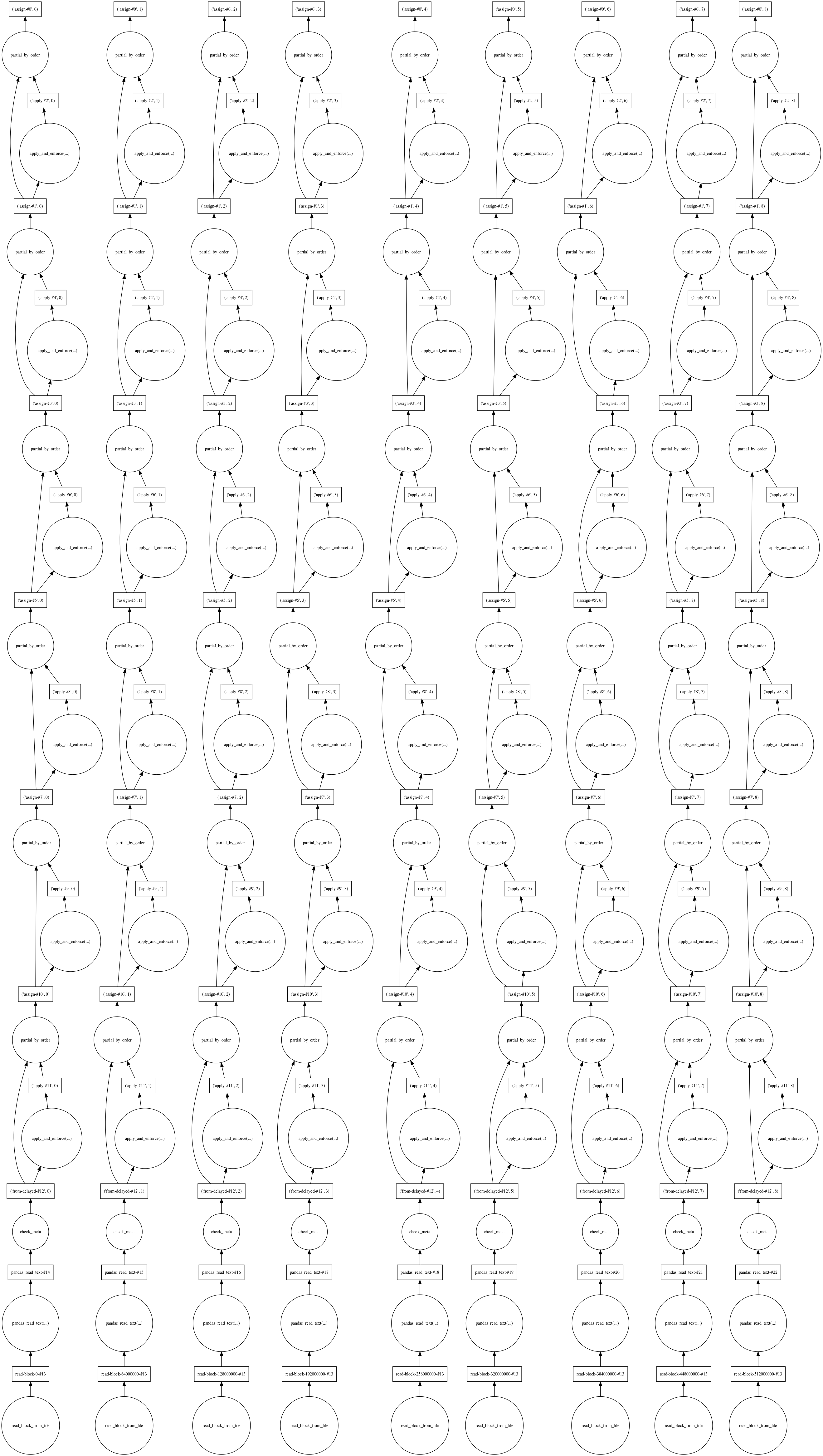
Below we execute all the column merge and the column drop operations that we have queued so far. We store the resulting DataFrame in a new variable.
if 'hurricanes_merged' not in os.listdir(data_dir):
    os.mkdir(os.path.join(data_dir,'hurricanes_merged'))

merged_csv_path = os.path.join(data_dir, 'hurricanes_merged')
Please note that the merge operation below might take about one hour. If you do not want to run the cell below, preprocessed data has been provided in sample data.
merged_df = full_df.drop(columns_to_drop, axis=1)
merged_df.to_csv(os.path.join(merged_csv_path, 'hurr_dask_*.csv'))
CPU times: user 43min 46s, sys: 6min 3s, total: 49min 49s Wall time: 45min 45s
The save() operation spawns several workers that compute in parallel. Notice the ouput file name contains a wildcard (*). This allows Dask to both read data in chunks and write outputs in chunks. The save operation will result in creating a number of processed CSV files whose names are prefixed with hurr_dask and suffixed with a number.
Preview results
Once Dask realizes a delayed computation, it returns the result as an in-memory Pandas DataFrame object. Thus, the merged_df variable represents a Pandas DataFrame object with 348,703 records and 17 columns.
merged_df.shape(348703, 17)
Creating hurricane tracks using Geoanalytics
The data collected so far are a set of Point observations representing all hurricanes recorded in the last 169 years. To make sense of these points, we need to connect them together to create a track for each hurricane. This part of the notebook uses ArcGIS GeoAnalytics server to reconstruct such hurricane tracks. The GeoAnalytics server is capable of processing on massive datasets in a scalable and distributed fashion.
The DASK process merged redundant columns together and ouput a folder full of CSV files. The GeoAnalytics server is also capabale of accepting a folder of datasets as 1 dataset and working on them. Thus in this part, we register that folder as a datastore and on the GeoAnalytics server for processing.
Reconstruct tracks:
Reconstruct tracks is a type of data aggregation tool available in the arcgis.geoanalytics module. This tool works with a layer of point features or polygon features that are time enabled. It first determines which points belong to a track using an identification number or identification string. Using the time at each location, the tracks are ordered sequentially and transformed into a line representing the path of movement. The map below shows a subset of the point datasets.

Create a data store
For the GeoAnalytics server to process your big data, it needs the data to be registered as a data store. In our case, the data is in multiple CSV files and we will register the folder containing the files as a data store of type bigDataFileShare.
Let us connect to our Organization.
gis = GIS(url='https://pythonapi.playground.esri.com/portal', username='arcgis_python', password='amazing_arcgis_123')Get the geoanalytics datastores and search for the registered datasets:
# Query the data stores available
datastores = get_datastores()
bigdata_fileshares = datastores.search()
bigdata_fileshares
[<Datastore title:"/enterpriseDatabases/AGSDataStore_ds_41yu9aqv" type:"egdb">, <Datastore title:"/bigDataFileShares/hurricanes_dask_csv" type:"bigDataFileShare">, <Datastore title:"/nosqlDatabases/AGSDataStore_nosqldb_tcs_yjayxzc4" type:"nosql">, <Datastore title:"/nosqlDatabases/AGSDataStore_bigdata_bds_wuqp7mbg" type:"nosql">, <Datastore title:"/rasterStores/LocalRasterDS" type:"rasterStore">]
The dataset hurricanes_dask_csv data is registered as a big data file share with the Geoanalytics datastore, so we can reference it:
data_item = bigdata_fileshares[1]If there is no big data file share for hurricane track data registered on the server, we can register one that points to the shared folder containing the CSV files.
data_item = datastores.add_bigdata("Hurricane_tracks", r"\\path_to_hurricane_data")Once a big data file share is registered, the GeoAnalytics server processes all the valid file types to discern the schema of the data, including information about the geometry in a dataset. If the dataset is time-enabled, as is required to use some GeoAnalytics Tools, the manifest reports the necessary metadata about how time information is stored as well.
This process can take a few minutes depending on the size of your data. Once processed, querying the manifest property will return a schema. As you can see from below, the schema contains the columns we merged using DASK previously.
datasets = data_item.manifest['datasets']
len(datasets)
1
[dataset['name'] for dataset in datasets]['hurricanes_merged']
datasets[0]{'name': 'hurricanes_merged',
'format': {'quoteChar': '"',
'fieldDelimiter': ',',
'hasHeaderRow': True,
'encoding': 'UTF-8',
'escapeChar': '"',
'recordTerminator': '\n',
'type': 'delimited',
'extension': 'csv'},
'schema': {'fields': [{'name': 'col_1', 'type': 'esriFieldTypeBigInteger'},
{'name': 'Serial_Num', 'type': 'esriFieldTypeString'},
{'name': 'Season', 'type': 'esriFieldTypeBigInteger'},
{'name': 'Num', 'type': 'esriFieldTypeBigInteger'},
{'name': 'Basin', 'type': 'esriFieldTypeString'},
{'name': 'Sub_basin', 'type': 'esriFieldTypeString'},
{'name': 'Name', 'type': 'esriFieldTypeString'},
{'name': 'ISO_time', 'type': 'esriFieldTypeString'},
{'name': 'Nature', 'type': 'esriFieldTypeString'},
{'name': 'Center', 'type': 'esriFieldTypeString'},
{'name': 'Track_type', 'type': 'esriFieldTypeString'},
{'name': 'Current Basin', 'type': 'esriFieldTypeString'},
{'name': 'latitude_merged', 'type': 'esriFieldTypeDouble'},
{'name': 'longitude_merged', 'type': 'esriFieldTypeDouble'},
{'name': 'wind_merged', 'type': 'esriFieldTypeDouble'},
{'name': 'pressure_merged', 'type': 'esriFieldTypeDouble'},
{'name': 'grade_merged', 'type': 'esriFieldTypeDouble'},
{'name': 'eye_dia_merged', 'type': 'esriFieldTypeDouble'}]},
'geometry': {'geometryType': 'esriGeometryPoint',
'spatialReference': {'wkid': 4326},
'fields': [{'name': 'longitude_merged', 'formats': ['x']},
{'name': 'latitude_merged', 'formats': ['y']}]},
'time': {'timeType': 'instant',
'fields': [{'name': 'ISO_time', 'formats': ['yyyy-MM-dd HH:mm:ss']}],
'timeReference': {'timeZone': 'UTC'}}}Perform data aggregation using reconstruct tracks tool
When you add a big data file share, a corresponding item gets created in your GIS. You can search for it like a regular item and query its layers.
search_result = gis.content.search("bigDataFileShares_hurricanes_dask_csv", item_type = "big data file share")
search_result
[<Item title:"bigDataFileShares_hurricanes_dask_csv" type:Big Data File Share owner:amani001>]
data_item = search_result[0]
cleaned_csv = data_item.layers[0]
cleaned_csv
<Layer url:"https://datascience-arcpy.esri.com/server/rest/services/DataStoreCatalogs/bigDataFileShares_hurricanes_dask_csv/BigDataCatalogServer/hurricanes_merged">
Execute reconstruct tracks tool
The reconstruct_tracks() function is available in the arcgis.geoanalytics.summarize_data module. In this example, we are using this tool to aggregate the numerous points into line segments showing the tracks followed by the hurricanes. The tool creates a feature layer item as an output which can be accessed once the processing is complete.
agg_result = reconstruct_tracks(cleaned_csv,
                                track_fields='Serial_Num',   # the Hurricane id number
                                method='GEODESIC', output_name='hurricane_tracks_aggregated_ga')
Submitted.
Executing...
Executing (ReconstructTracks): ReconstructTracks "Feature Set" Serial_Num Geodesic # # # # # # "{"serviceProperties": {"name": "hurricane_tracks_aggregated_ga", "serviceUrl": "https://datascience-arcpy.esri.com/server/rest/services/Hosted/hurricane_tracks_aggregated_ga/FeatureServer"}, "itemProperties": {"itemId": "545adb07c4ba4da7b72ddbe47bd275d2"}}" "{"defaultAggregationStyles": false}"
Start Time: Thu Nov 15 21:57:30 2018
Using URL based GPRecordSet param: https://datascience-arcpy.esri.com/server/rest/services/DataStoreCatalogs/bigDataFileShares_hurricanes_dask_csv/BigDataCatalogServer/hurricanes_merged
{"messageCode":"BD_101028","message":"Starting new distributed job with 352 tasks.","params":{"totalTasks":"352"}}
{"messageCode":"BD_101029","message":"0/352 distributed tasks completed.","params":{"completedTasks":"0","totalTasks":"352"}}
{"messageCode":"BD_101029","message":"177/352 distributed tasks completed.","params":{"completedTasks":"177","totalTasks":"352"}}
{"messageCode":"BD_101029","message":"241/352 distributed tasks completed.","params":{"completedTasks":"241","totalTasks":"352"}}
{"messageCode":"BD_101029","message":"308/352 distributed tasks completed.","params":{"completedTasks":"308","totalTasks":"352"}}
{"messageCode":"BD_101029","message":"352/352 distributed tasks completed.","params":{"completedTasks":"352","totalTasks":"352"}}
{"messageCode":"BD_101081","message":"Finished writing results:"}
{"messageCode":"BD_101082","message":"* Count of features = 12757","params":{"resultCount":"12757"}}
{"messageCode":"BD_101083","message":"* Spatial extent = {\"xmin\":-180,\"ymin\":-68.5,\"xmax\":180,\"ymax\":81}","params":{"extent":"{\"xmin\":-180,\"ymin\":-68.5,\"xmax\":180,\"ymax\":81}"}}
{"messageCode":"BD_101084","message":"* Temporal extent = Interval(MutableInstant(1842-10-25 06:00:00.000),MutableInstant(2017-06-13 06:00:00.000))","params":{"extent":"Interval(MutableInstant(1842-10-25 06:00:00.000),MutableInstant(2017-06-13 06:00:00.000))"}}
{"messageCode":"BD_101054","message":"Some records have either missing or invalid geometries."}
{"messageCode":"BD_101054","message":"Some records have either missing or invalid geometries."}
Succeeded at Thu Nov 15 21:57:54 2018 (Elapsed Time: 24.21 seconds)
Analyze the result of aggregation
The reconstruct tracks produces summary statistics such as MIN, MAX, MEAN, MEDIAN, RANGE, SD, VAR, SUM, for numeric columns and COUNT for ordinal columns during the aggregation process. Let us list the fields in this dataset to view them.
agg_tracks_layer = agg_result.layers[0]
agg_fields = [f.name for f in agg_tracks_layer.properties.fields]
pprint(agg_fields, compact=True)
['Serial_Num', 'COUNT', 'COUNT_col_1', 'SUM_col_1', 'MIN_col_1', 'MAX_col_1', 'MEAN_col_1', 'RANGE_col_1', 'SD_col_1', 'VAR_col_1', 'COUNT_Season', 'SUM_Season', 'MIN_Season', 'MAX_Season', 'MEAN_Season', 'RANGE_Season', 'SD_Season', 'VAR_Season', 'COUNT_Num', 'SUM_Num', 'MIN_Num', 'MAX_Num', 'MEAN_Num', 'RANGE_Num', 'SD_Num', 'VAR_Num', 'COUNT_Basin', 'ANY_Basin', 'COUNT_Sub_basin', 'ANY_Sub_basin', 'COUNT_Name', 'ANY_Name', 'COUNT_ISO_time', 'ANY_ISO_time', 'COUNT_Nature', 'ANY_Nature', 'COUNT_Center', 'ANY_Center', 'COUNT_Track_type', 'ANY_Track_type', 'COUNT_Current_Basin', 'ANY_Current_Basin', 'COUNT_latitude_merged', 'SUM_latitude_merged', 'MIN_latitude_merged', 'MAX_latitude_merged', 'MEAN_latitude_merged', 'RANGE_latitude_merged', 'SD_latitude_merged', 'VAR_latitude_merged', 'COUNT_longitude_merged', 'SUM_longitude_merged', 'MIN_longitude_merged', 'MAX_longitude_merged', 'MEAN_longitude_merged', 'RANGE_longitude_merged', 'SD_longitude_merged', 'VAR_longitude_merged', 'COUNT_wind_merged', 'SUM_wind_merged', 'MIN_wind_merged', 'MAX_wind_merged', 'MEAN_wind_merged', 'RANGE_wind_merged', 'SD_wind_merged', 'VAR_wind_merged', 'COUNT_pressure_merged', 'SUM_pressure_merged', 'MIN_pressure_merged', 'MAX_pressure_merged', 'MEAN_pressure_merged', 'RANGE_pressure_merged', 'SD_pressure_merged', 'VAR_pressure_merged', 'COUNT_grade_merged', 'SUM_grade_merged', 'MIN_grade_merged', 'MAX_grade_merged', 'MEAN_grade_merged', 'RANGE_grade_merged', 'SD_grade_merged', 'VAR_grade_merged', 'COUNT_eye_dia_merged', 'SUM_eye_dia_merged', 'MIN_eye_dia_merged', 'MAX_eye_dia_merged', 'MEAN_eye_dia_merged', 'RANGE_eye_dia_merged', 'SD_eye_dia_merged', 'VAR_eye_dia_merged', 'TRACK_DURATION', 'globalid', 'OBJECTID', 'END_DATETIME', 'START_DATETIME']
To get the number of hurricanes the reconstruct tracks tool identified, we run a query on the aggregation layer and get just the number of records.
agg_tracks_layer.query(return_count_only=True)12362
Conclusion
In this notebook, we observed how to download meteorological data over FTP from NEIC website. The data came in 169 CSV files for the past 169 years. We sanitized it initially using Pandas to remove bad header rows. We then used DASK library to read all 169 files as a single file and merged data from redundant columns. This pre-processing resulted in multiple output CSV files covering a total of 348k records and 17 columns.
This data was fed to the ArcGIS GeoAnalytics server for aggregation. The reconstruct tracks tool on GeoAnalytics server reduced this point dataset into hurricane tracks (lines) and during this aggregation, it calculated summary statistics for the numerical columns. The tool identified 12,362 individual hurricanes from the past 169 years.
In Part 2 of this study, we will visualize and explore this dataset to understand the prevelance, duration of hurricanes and the communities affected by hurricanes worldwide.
In Part 3, we will analyze this aggregated result comprehensively, answer important questions such as, does the intensity of hurricanes increase over time and draw conclusions.