Buying or selling of a house can be a very stressful event in one's life. The process could be frustrating as it is lengthy, uncertain and needs a lot of examination. Through this workflow we will guide a couple (Mark and Lisa) who is interested in selling their home and relocating to a place nearest to both of their work places. In this case study, we will explore the current housing market, estimate average house prices in their area and hunt for a new one. We will download the Zillow data for their current home for our analysis. You can use your own data and follow along with this workflow which aims to help Mark and Lisa in finding their new home.

The notebook is divided into two parts. In the first part, we will calculate the following:
- Percentage of decrease/increase in house price since Mark and Lisa bought their home.
- Suggested selling price for their home.
- Whether their zip code is a buyer’s market or seller’s market.
- Average number of days it takes for homes to sell in their neighbourhood.
In the second part of the notebook, we will explore the investment potential of homes close to their work places. Based on how much a person is willing to spend commuting to work, we will create a drive-time buffer. This will narrow down the search areas. Zillow also provides data for market health and projected home value appreciation. Visualizing the zip codes by their market health will help them focus only on areas with good market health. Hence they will get a list of areas to choose from, for buying their new home.
Selling your home
Execute the following command to install the openpyxl library if not already. This package is used to read from any Excel or CSV files.
!pip install openpyxl
Also, when matplotlib is not present, run the following command to have it installed or upgraded:
import sys
!{sys.executable} -m pip install matplotlib
Determine an appropriate selling price
1) Download home sales time series data from Zillow at www.zillow.com/research/data.
Mark and Lisa have a 3-bedroom home, so we will select the ZHVI 3-Bedroom time-series ($) data set at the ZIP Code level.
2) Prepare the Excel data as follows:
a) Using Excel, open the .csv file.
Notice that the RegionName field has ZIP Codes as numbers (if we sort the RegionName field we will notice the ZIP Codes for Massachusetts, for example, don't have leading zeros; 01001 is 1001). Also, notice the median home value columns are named using the year and month. The first data available is for April 1996 (1996-04). b) Copy all the column headings and the one record with data for their ZIP Code to a new Excel sheet.
Apply a filter to the RegionName field. Mark and Lisa live in Crestline, California, so we will apply a filter for the 92325 ZIP Code.

c) Select (highlight) fields starting with the month and year when they bought their home and continuing to the last month and year column in the Excel table. So, for example, since Mark and Lisa bought their home in December 2007, they highlight the the two rows from column 2007-01 to column 2018-08.
d) Copy (press Ctrl+C) the selected data and paste it, along with the column headings, to a new Excel sheet using Paste Transposed (right-click in the first cell of the new sheet to see the paste options; select Paste Transposed). This gives two columns of data.
e) The first column has date values but only includes the year and month. In column C, create a proper date field.
- Right-click column C and format the cells to be category date.
- In the first cell of column C, enter the following formula: = DATEVALUE(CONCATENATE(A1, "-01"))
- Drag the Autofill handle down to the last data cell in the column.
f) Insert a top row and type the column headings:
YYYYMM, Value, and date.

g) Rename the Excel sheet (probably called Sheet2 at present) something like
AveSellingPrice and delete the other sheets (the first sheet contains a large amount of data that we won't be using further in the workflow).
Mark and Lisa named their price Excel sheet CrestlineAveSellingPrice.
h) Save this new sheet as an Excel workbook.
Mark and Lisa named their Excel file Crestline3BdrmAveSellingPrice.xlsx.
3) Connect to your ArcGIS Online organization.
from arcgis.gis import GISimport pandas as pd
import matplotlib.pyplot as plt
from datetime import datetime as dtgis = GIS('home')Use the boolean has_arcpy to flag whether arcpy is present on the local environement:
has_arcpy = Falsetry:
import arcpy
has_arcpy = True
print("arcpy present")
except:
print("arcpy not present")arcpy not present
4) Load the excel file for analysis.
data = gis.content.search('finding_a_new_home owner:api_data_owner type: csv collection')[0]
data
filepath = data.download(file_name=data.name)import os
import zipfile
from pathlib import Path
with zipfile.ZipFile(filepath, 'r') as zip_ref:
zip_ref.extractall(Path(filepath).parent)data_path = Path(os.path.join(os.path.splitext(filepath)[0]))
data_pathWindowsPath('C:/Users/pri10421/AppData/Local/Temp/finding_a_new_home')datapath = [os.path.abspath(os.path.join(data_path, p)) for p in os.listdir(data_path)]
datapath['C:\\Users\\pri10421\\AppData\\Local\\Temp\\finding_a_new_home\\BuyerSellerIndex.xlsx', 'C:\\Users\\pri10421\\AppData\\Local\\Temp\\finding_a_new_home\\Crestline3BdrmAveSellingPrice.xlsx', 'C:\\Users\\pri10421\\AppData\\Local\\Temp\\finding_a_new_home\\ImportantPlaces.xlsx', 'C:\\Users\\pri10421\\AppData\\Local\\Temp\\finding_a_new_home\\MarketHealthIndex.xlsx']
file_name1 = datapath[1]
data1 = pd.pandas.read_excel(file_name1)data1.head()| YYYYMM | value | date | |
|---|---|---|---|
| 0 | 2007-01 | 291000 | 2007-01-01 |
| 1 | 2007-02 | 289000 | 2007-02-01 |
| 2 | 2007-03 | 287400 | 2007-03-01 |
| 3 | 2007-04 | 286100 | 2007-04-01 |
| 4 | 2007-05 | 284000 | 2007-05-01 |
data1.tail()| YYYYMM | value | date | |
|---|---|---|---|
| 135 | 2018-04 | 252200 | 2018-04-01 |
| 136 | 2018-05 | 254000 | 2018-05-01 |
| 137 | 2018-06 | 254800 | 2018-06-01 |
| 138 | 2018-07 | 254900 | 2018-07-01 |
| 139 | 2018-08 | 254900 | 2018-08-01 |
data1.shape(140, 3)
data1[['year','month','day']] = data1.date.apply(lambda x: pd.Series(
x.strftime("%Y,%m,%d").split(","))) # split date into year, month, daydata1.head()| YYYYMM | value | date | year | month | day | |
|---|---|---|---|---|---|---|
| 0 | 2007-01 | 291000 | 2007-01-01 | 2007 | 01 | 01 |
| 1 | 2007-02 | 289000 | 2007-02-01 | 2007 | 02 | 01 |
| 2 | 2007-03 | 287400 | 2007-03-01 | 2007 | 03 | 01 |
| 3 | 2007-04 | 286100 | 2007-04-01 | 2007 | 04 | 01 |
| 4 | 2007-05 | 284000 | 2007-05-01 | 2007 | 05 | 01 |
grpby_data1 = data1.groupby(['year']).mean()type(grpby_data1)pandas.core.frame.DataFrame
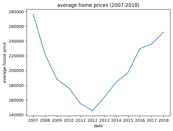
5) We will Create a graph showing how average home prices have changed since they bought their home.
grpby_data1.reset_index(inplace=True)grpby_data1.head()| year | value | |
|---|---|---|
| 0 | 2007 | 276616.666667 |
| 1 | 2008 | 221875.000000 |
| 2 | 2009 | 188391.666667 |
| 3 | 2010 | 176216.666667 |
| 4 | 2011 | 154766.666667 |
grpby_data1.value0 276616.666667 1 221875.000000 2 188391.666667 3 176216.666667 4 154766.666667 5 145158.333333 6 163741.666667 7 183975.000000 8 197133.333333 9 229566.666667 10 235966.666667 11 252025.000000 Name: value, dtype: float64
grpby_data1.year0 2007 1 2008 2 2009 3 2010 4 2011 5 2012 6 2013 7 2014 8 2015 9 2016 10 2017 11 2018 Name: year, dtype: object
plt.plot(grpby_data1.year, grpby_data1.value)
plt.title("average home prices (2007-2018)")
plt.xlabel("date")
plt.ylabel("average house price")
Text(0, 0.5, 'average house price')
7) Determine an appropriate selling price based on home sales trends as follows:
a) Determine the current average selling price and the average selling price when they bought their home. Divide the current average price by the beginning average price to see how much homes in their ZIP Code have appreciated or depreciated. When Mark and Lisa bought their home in December of 2007, 3-bedroom homes were selling for \$276,617.
price_initial = grpby_data1.iloc[0]price_initialyear 2007 value 276616.666667 Name: 0, dtype: object
price_current = grpby_data1.iloc[-1]price_currentyear 2018 value 252025.0 Name: 11, dtype: object
house_worth = price_current.value / price_initial.valuehouse_worth0.9110983912755316
This indicates that homes in Crestline are only worth 91 percent of what they were at the end of 2007.
b) We can get a rough estimate of what their home is worth by summing what they paid for their home plus what they invested in it, and multiplying that sum by the ratio computed above. Mark and Lisa, for example, paid \$291,000 in 2007 and invested \$100,000 in solid improvements (new kitchen, major landscaping, hardwood flooring, and so on). Multiplying (\$291,000 + \$100,000) by 0.91 gives a rough suggested selling price of \$343,134.
(price_initial.value + 100000)*house_worth343134.83912755316
Get additional information about the local real estate market
If their home is part of a seller's market, they are more likely to get their asking price.
1) Download the Buyer-Seller Index data at the ZIP Code level from www.zillow.com/research/data. In Home Listings and Sales select data type as seller-buyer index and geography as zip codes.
2) Open the .csv file using Excel. Zillow reports ZIP Codes as numbers. We will need to pad the ZIP Code numbers with leading zeros so the Zillow data will link to the ArcGIS ZIP Code geometry.
Follow these steps:
a) Sort the RegionName column from smallest to largest so we will be able to see how the formula below works.
b) Name a new column in the Excel table zipstring.
c) In the first cell of the new column, enter the formula to pad each RegionName value with leading zeros, keeping the rightmost five characters: =RIGHT(CONCAT("00000",B2),5)
d) Drag the Autofill handle down to the last data cell in the column.


3) Load the excel file for analysis
file_name2 = datapath[0]
data2 = pd.read_excel(file_name2)data2.head()| RegionType | RegionName | State | CBSA Title | SizeRankCity | SizeRankMetro | PctPriceCut | DaysOnMarket | BuyerSellerIndex | BuyerSellerIndexMetro | zipstring | |
|---|---|---|---|---|---|---|---|---|---|---|---|
| 0 | Zip | 1001 | MA | Springfield, MA | 8273 | 83 | 22.916667 | 81.0 | 6.190476 | 9.185083 | 1001 |
| 1 | Zip | 1002 | MA | Springfield, MA | 6684 | 83 | 29.787234 | 94.0 | 10.000000 | 9.185083 | 1002 |
| 2 | Zip | 1007 | MA | Springfield, MA | 9088 | 83 | 16.091954 | 83.0 | 2.857143 | 9.185083 | 1007 |
| 3 | Zip | 1013 | MA | Springfield, MA | 7061 | 83 | 31.147541 | 76.5 | 8.333333 | 9.185083 | 1013 |
| 4 | Zip | 1020 | MA | Springfield, MA | 5172 | 83 | 25.000000 | 73.0 | 3.809524 | 9.185083 | 1020 |
data2.dtypesRegionType object RegionName int64 State object CBSA Title object SizeRankCity int64 SizeRankMetro int64 PctPriceCut float64 DaysOnMarket float64 BuyerSellerIndex float64 BuyerSellerIndexMetro float64 zipstring int64 dtype: object
data2.columnsIndex(['RegionType', 'RegionName', 'State', 'CBSA Title', 'SizeRankCity',
'SizeRankMetro', 'PctPriceCut', 'DaysOnMarket', 'BuyerSellerIndex',
'BuyerSellerIndexMetro', 'zipstring'],
dtype='object')4) Select BuyerSellerIndex, DaysOnMarket, zipstring fields
cols = ['BuyerSellerIndex', 'DaysOnMarket', 'zipstring']selected_data2 = data2[cols]5) Explore the data values as follows:
a) Sort on the DaysOnMarket field and notice the range. For the data Mark and Lisa downloaded, the range is 35 to 294.5 days.
days_on_mrkt_df = selected_data2.sort_values(by='DaysOnMarket', axis=0)days_on_mrkt_df.DaysOnMarket.min()35.0
days_on_mrkt_df.DaysOnMarket.max()294.5
days_on_mrkt_df.head()| BuyerSellerIndex | DaysOnMarket | zipstring | |
|---|---|---|---|
| 7420 | 1.120000 | 35.0 | 98107 |
| 7434 | 4.960000 | 35.0 | 98136 |
| 7097 | 0.526316 | 35.0 | 94022 |
| 7426 | 0.640000 | 35.0 | 98117 |
| 7399 | 0.080000 | 35.0 | 98043 |
days_on_mrkt_df.tail()| BuyerSellerIndex | DaysOnMarket | zipstring | |
|---|---|---|---|
| 800 | 9.006849 | 252.0 | 8752 |
| 1177 | 10.000000 | 254.0 | 12428 |
| 1141 | 8.938356 | 261.5 | 11963 |
| 1189 | 9.160959 | 288.0 | 12545 |
| 753 | 6.000000 | 294.5 | 8403 |
b) Sort on the BuyerSellerIndex field and notice the range of values. ZIP Codes with index values near 0 are part of a strong seller's market; ZIP Codes with index values near 10 are part of a strong buyer's market.
buyer_seller_df = data2.sort_values(by='BuyerSellerIndex', axis=0)buyer_seller_df.head()| RegionType | RegionName | State | CBSA Title | SizeRankCity | SizeRankMetro | PctPriceCut | DaysOnMarket | BuyerSellerIndex | BuyerSellerIndexMetro | zipstring | |
|---|---|---|---|---|---|---|---|---|---|---|---|
| 517 | Zip | 7063 | NJ | New York-Newark-Jersey City, NY-NJ-PA | 10423 | 1 | 4.687500 | 90.0 | 0.017123 | 9.585635 | 7063 |
| 4546 | Zip | 53168 | WI | Chicago-Naperville-Elgin, IL-IN-WI | 10505 | 3 | 9.756098 | 59.5 | 0.033223 | 9.488950 | 53168 |
| 485 | Zip | 7004 | NJ | New York-Newark-Jersey City, NY-NJ-PA | 10846 | 1 | 7.894737 | 92.0 | 0.034247 | 9.585635 | 7004 |
| 6572 | Zip | 90025 | CA | Los Angeles-Long Beach-Anaheim, CA | 2122 | 2 | 6.451613 | 46.0 | 0.036364 | 4.185083 | 90025 |
| 1609 | Zip | 19152 | PA | Philadelphia-Camden-Wilmington, PA-NJ-DE-MD | 4927 | 5 | 6.818182 | 67.0 | 0.041667 | 9.150552 | 19152 |
buyer_seller_df.tail()| RegionType | RegionName | State | CBSA Title | SizeRankCity | SizeRankMetro | PctPriceCut | DaysOnMarket | BuyerSellerIndex | BuyerSellerIndexMetro | zipstring | |
|---|---|---|---|---|---|---|---|---|---|---|---|
| 6091 | Zip | 80016 | CO | Denver-Aurora-Lakewood, CO | 2658 | 21 | 27.226891 | 62.0 | 10.0 | 4.502762 | 80016 |
| 4598 | Zip | 53954 | WI | Madison, WI | 10773 | 87 | 21.875000 | 75.5 | 10.0 | 3.522099 | 53954 |
| 262 | Zip | 3049 | NH | Manchester-Nashua, NH | 10693 | 131 | 28.787879 | 74.0 | 10.0 | 3.577348 | 3049 |
| 7321 | Zip | 97209 | OR | Portland-Vancouver-Hillsboro, OR-WA | 4742 | 23 | 26.258993 | 78.5 | 10.0 | 5.096685 | 97209 |
| 1224 | Zip | 13104 | NY | Syracuse, NY | 8916 | 79 | 28.323699 | 89.0 | 10.0 | 9.033149 | 13104 |
buyer_seller_df.BuyerSellerIndex.min()0.017123288
buyer_seller_df.BuyerSellerIndex.max()10.0
c) Filter the data to only show their home's ZIP code
selected_data2[selected_data2['zipstring'] == 92325]| BuyerSellerIndex | DaysOnMarket | zipstring | |
|---|---|---|---|
| 6888 | 9.622642 | 79.0 | 92325 |
Notice the average number of days. Determine if the home is part of a buyer's or seller's market. Mark and Lisa learn that their home is part of a buyer's market (9.6), and they can expect their home to be on the market approximately 79 days before it sells.
selected_data2.rename(columns={"zipstring": "ZIP_CODE"}, inplace=True)C:\Users\pri10421\AppData\Local\Temp\ipykernel_17192\3169181311.py:1: SettingWithCopyWarning:
A value is trying to be set on a copy of a slice from a DataFrame
See the caveats in the documentation: https://pandas.pydata.org/pandas-docs/stable/user_guide/indexing.html#returning-a-view-versus-a-copy
selected_data2.rename(columns={"zipstring": "ZIP_CODE"}, inplace=True)
selected_data2.shape(7548, 3)
selected_data2.dtypesBuyerSellerIndex float64 DaysOnMarket float64 ZIP_CODE int64 dtype: object
selected_data2 = selected_data2.astype({"ZIP_CODE": int})selected_data2.dtypesBuyerSellerIndex float64 DaysOnMarket float64 ZIP_CODE int32 dtype: object
6) Search for the United States ZIP Code Boundaries 2017 layer. We can specify the owner's name to get more specific results. To search for content from the Living Atlas, or content shared by other users on ArcGIS Online, set outside_org=True
items = gis.content.search('United States ZIP Code Boundaries 2021 owner: esri_dm',
                           outside_org=True)
Display the list of results.
from IPython.display import display

for item in items:
    display(item)


Select the desired item from the list.
us_zip = items[1]us_zip
Get the layer names from the item
for lyr in us_zip.layers:
    print(lyr.properties.name)
USA_Country USA_State USA_County USA_ZipCode USA_Tract USA_BlockGroup
7) We want to merge the zip_code layer with data2 to visualize the result on the map.
us_zip_lyr = us_zip.layers[3]zip_df = pd.DataFrame.spatial.from_layer(us_zip_lyr)zip_df.head()| OBJECTID | POPULATION | PO_NAME | SHAPE | SQMI | STATE | Shape__Area | Shape__Length | ZIP_CODE | |
|---|---|---|---|---|---|---|---|---|---|
| 0 | 1 | <NA> | N Dillingham Census Area | {"rings": [[[-160.431152, 58.689351], [-160.43... | 16019.53 | AK | 6.657141 | 24.677454 | 00001 |
| 1 | 2 | <NA> | Yukon Flats Nat Wildlife | {"rings": [[[-160.038452, 61.947605], [-160.03... | 95862.85 | AK | 48.948815 | 131.77645 | 00002 |
| 2 | 3 | <NA> | Alaska Peninsula NWR | {"rings": [[[-159.900745, 56.439047], [-159.90... | 14572.9 | AK | 5.655405 | 41.564165 | 00003 |
| 3 | 4 | <NA> | W Kenai Peninsula Borough | {"rings": [[[-154.748861, 59.259518], [-154.70... | 6510.85 | AK | 2.728764 | 20.553203 | 00004 |
| 4 | 5 | <NA> | N Lake and Peninsula Borough | {"rings": [[[-156.0002144, 60.9074352], [-155.... | 3760.07 | AK | 1.593722 | 9.571684 | 00005 |
zip_df.shape(32201, 9)
zip_df.dtypesOBJECTID Int64 POPULATION Int32 PO_NAME string SHAPE geometry SQMI Float64 STATE string Shape__Area Float64 Shape__Length Float64 ZIP_CODE string dtype: object
zip_df = zip_df.astype({"ZIP_CODE": int})zip_df.dtypesOBJECTID Int64 POPULATION Int32 PO_NAME string SHAPE geometry SQMI Float64 STATE string Shape__Area Float64 Shape__Length Float64 ZIP_CODE int32 dtype: object
merged_df = pd.merge(zip_df, selected_data2, on='ZIP_CODE')merged_df.shape(7548, 11)
merged_df.spatial.set_geometry('SHAPE')mergd_lyr = gis.content.import_data(merged_df,
title='MergedLayer',
tags='datascience')When arcpy is present, the import_data will upload the local SeDF (Spatially Enabled DataFrame) as a FGDB (File geodatabase) to your organization, and publish to a hosted feature layer; On the other hand, when arcpy is not present, then the import_data method would have the local SeDF upload to your organization as a shapefile, and then publish as a hosted Feature Layer. This minor difference will result in column/property name differences from what's defined in the original SeDF.
The has_arcpy flag is to be used in determine which naming convention the newly created Feature Layer would be conforming to, when we are adding the Feature Layer for display based on variables.
8) Create a map of the BuyerSellerIndex field using the following steps:
Visualize Results
m1 = gis.map('United States', 8)
m1
cur_field_name = "BuyerSellerIndex"
if has_arcpy:
    if cur_field_name not in mergd_lyr.layers[0].properties.fields:
        cur_field_name = "buyer_seller_index"
else:
    cur_field_name = "BuyerSelle"
m1.add_layer(mergd_lyr, {"renderer":"ClassedColorRenderer",
"field_name":cur_field_name,
"opacity":0.7
})9) Create a map on DaysOnMarket field as follows:
m2 = gis.map('Redlands, CA')
m2
cur_field_name = "DaysOnMarket"
if has_arcpy:
    if cur_field_name not in mergd_lyr.layers[0].properties.fields:
        cur_field_name = "days_on_market"
else:
    cur_field_name = "DaysOnMark"
m2.add_layer(mergd_lyr, {"renderer":"ClassedSizeRenderer",
"field_name":cur_field_name,
"opacity":0.7
})House Hunting
Find all ZIP Codes within a specified drive time of important places
1) Create an Excel table with columns for Street, City, State, and Zip. Add addresses for the locations you want to access from your new home. Mark and Lisa's table below has their current job addresses. They named their Excel file ImportantPlaces.xlsx and the Excel sheet WorkLocations.
2) Load the excel file for analysis
file_name3 = datapath[2]
data3 = pd.read_excel(file_name3)data3.head()| Place | Street | City | State | Zip | |
|---|---|---|---|---|---|
| 0 | Lisa's job | 380 New York Street | Redlands | CA | 92373 |
| 1 | Mark's job | 4511 E Guasti Road | Ontario | CA | 91761 |
data3['Address'] = data3['Street'] + ' ' + data3['City'] + ' ' + data3['State']data3['Address']0 380 New York Street Redlands CA 1 4511 E Guasti Road Ontario CA Name: Address, dtype: object
3) Draw the address on map
m3 = gis.map('Redlands, CA', 10)
m3
from arcgis.geocoding import geocode
data3_addr1 = geocode(data3.Address[0])[0]
popup = {
    "title" : "Lisa's job",
    "content" : data3_addr1['address']
    }
m3.draw(data3_addr1['location'], popup,
        symbol = {"angle":0,"xoffset":0,"yoffset":0,
                  "type":"esriPMS", "url":"https://static.arcgis.com/images/Symbols/PeoplePlaces/School.png",
                  "contentType":"image/png","width":24,"height":24})
from arcgis.geocoding import geocode
data3_addr2 = geocode(data3.Address[1])[0]
popup = {
"title" : "Mark's job",
"content" : data3_addr2['address']
}
m3.draw(data3_addr2['location'], popup,
symbol = {"angle":0,"xoffset":0,"yoffset":0,
"type":"esriPMS", "url":"https://static.arcgis.com/images/Symbols/PeoplePlaces/School.png",
"contentType":"image/png","width":24,"height":24})4) We will Create buffer and enter the maximum time they are willing to spend commuting from their new home to their work.
from arcgis.geoenrichment import BufferStudyArea, enrichmarks = BufferStudyArea(area='4511 E Guasti Road, Ontario, CA 91761',
radii=[45], units='Minutes',
travel_mode='Driving')
lisas = BufferStudyArea(area='380 New York St Redlands CA 92373',
radii=[45], units='Minutes',
travel_mode='Driving')
drive_time_df = enrich(study_areas=[marks, lisas], data_collections=['Age'])drive_time_lyr = gis.content.import_data(drive_time_df,
title="DriveTimeLayer")5) Select the Dissolve buffer style to merge overlapping polygons.
from arcgis.features.manage_data import dissolve_boundariesdissolved_lyr = dissolve_boundaries(drive_time_lyr)m_3 = gis.map('Redlands, CA', 9)
m_3
m_3.add_layer(dissolved_lyr)m_3.draw(data3_addr1['location'], popup,
symbol = {"angle":0,"xoffset":0,"yoffset":0,
"type":"esriPMS", "url":"https://static.arcgis.com/images/Symbols/PeoplePlaces/School.png",
"contentType":"image/png","width":24,"height":24})
m_3.draw(data3_addr2['location'], popup,
symbol = {"angle":0,"xoffset":0,"yoffset":0,
"type":"esriPMS", "url":"https://static.arcgis.com/images/Symbols/PeoplePlaces/School.png",
"contentType":"image/png","width":24,"height":24})Map market health, home values, and projected appreciation
1) Download and prepare the Excel Market Health data as follows:
a) From www.zillow.com/reserach/data, download ZIP Code level Market Health Index data.
b) Open the .csv file using Excel and add the ZIPString column as a text field. Compute the values using =RIGHT(CONCAT("00000",B2),5). Drag the Autofill handle down to the last cell in the column to create text formatted ZIP Code values with leading zeros.
c) Save the file as an Excel workbook. Close Excel.
Mark and Lisa named their file MarketHealth.xlsx.
2) Load th Excel file for analysis.
file_name4 = datapath[3]
data4 = pd.read_excel(file_name4)data4| RegionType | RegionName | City | State | Metro | CBSATitle | SizeRank | MarketHealthIndex | SellForGain | PrevForeclosed | ... | ZHVI | MoM | YoY | ForecastYoYPctChange | StockOfREOs | NegativeEquity | Delinquency | DaysOnMarket | Unnamed: 19 | zipstring | |
|---|---|---|---|---|---|---|---|---|---|---|---|---|---|---|---|---|---|---|---|---|---|
| 0 | Zip | 1001 | Agawam | MA | Springfield, MA, MA | Springfield, MA | NaN | 1.622365 | 75.00 | 0.0500 | ... | 214000.0 | 0.281162 | 5.263158 | 0.047047 | NaN | 0.069028 | 0.068063 | 81.0 | NaN | 1001 |
| 1 | Zip | 1002 | Amherst | MA | Springfield, MA, MA | Springfield, MA | NaN | 5.491341 | 92.31 | 0.0000 | ... | 331400.0 | 0.485143 | 6.972240 | 0.046192 | NaN | 0.045415 | 0.038462 | 87.5 | NaN | 1002 |
| 2 | Zip | 1007 | Belchertown | MA | Springfield, MA, MA | Springfield, MA | NaN | 4.664384 | 100.00 | 0.0000 | ... | 277400.0 | 0.325497 | 4.679245 | 0.054387 | NaN | 0.046303 | 0.048387 | 94.5 | NaN | 1007 |
| 3 | Zip | 1008 | Blandford | MA | Springfield, MA, MA | Springfield, MA | NaN | 2.541281 | 0.00 | NaN | ... | 224000.0 | 0.223714 | 8.843537 | 0.061817 | NaN | 0.060109 | 0.090909 | 73.0 | NaN | 1008 |
| 4 | Zip | 1010 | Brimfield | MA | Springfield, MA, MA | Springfield, MA | NaN | 3.103101 | 100.00 | NaN | ... | 255700.0 | 0.471513 | 2.608347 | 0.060555 | NaN | 0.066778 | 0.075000 | 73.0 | NaN | 1010 |
| ... | ... | ... | ... | ... | ... | ... | ... | ... | ... | ... | ... | ... | ... | ... | ... | ... | ... | ... | ... | ... | ... |
| 14893 | Zip | 75033 | Frisco | TX | Dallas-Fort Worth, TX, TX | Dallas-Fort Worth, TX | NaN | 9.095852 | 100.00 | 0.0000 | ... | 395800.0 | -0.075738 | 1.046719 | 0.066809 | NaN | NaN | NaN | 74.0 | NaN | 75033 |
| 14894 | Zip | 84009 | South Jordan | UT | Salt Lake City, UT, UT | Salt Lake City, UT | NaN | 6.135052 | NaN | 0.0000 | ... | 409200.0 | 0.540541 | 9.120000 | 0.040208 | NaN | NaN | NaN | 48.0 | NaN | 84009 |
| 14895 | Zip | 97003 | Beaverton | OR | Portland, OR, OR | Portland, OR | NaN | 6.806954 | 100.00 | 0.0000 | ... | 346900.0 | 0.173260 | 5.376671 | 0.037766 | NaN | NaN | NaN | 44.0 | NaN | 97003 |
| 14896 | Zip | 97703 | Bend | OR | Bend, OR, OR | Bend, OR | NaN | 6.566653 | 100.00 | NaN | ... | 590700.0 | 0.288625 | 6.489995 | -0.011788 | NaN | NaN | NaN | 77.0 | NaN | 97703 |
| 14897 | Zip | 29486 | Summerville | SC | Charleston, SC, SC | Charleston, SC | NaN | 6.815009 | 91.30 | 0.0196 | ... | 192200.0 | 0.417973 | 7.314350 | 0.019964 | NaN | NaN | NaN | 83.5 | NaN | 29486 |
14898 rows × 21 columns
3) Select City, MarketHealthIndex, ZHVI, ForecastYoYPctChange, and zipstring fields.
col = ['City', 'MarketHealthIndex', 'ZHVI', 'ForecastYoYPctChange', 'zipstring']matket_health_index = data4[col]matket_health_index.head()| City | MarketHealthIndex | ZHVI | ForecastYoYPctChange | zipstring | |
|---|---|---|---|---|---|
| 0 | Agawam | 1.622365 | 214000.0 | 0.047047 | 1001 |
| 1 | Amherst | 5.491341 | 331400.0 | 0.046192 | 1002 |
| 2 | Belchertown | 4.664384 | 277400.0 | 0.054387 | 1007 |
| 3 | Blandford | 2.541281 | 224000.0 | 0.061817 | 1008 |
| 4 | Brimfield | 3.103101 | 255700.0 | 0.060555 | 1010 |
matket_health_index.dtypesCity object MarketHealthIndex float64 ZHVI float64 ForecastYoYPctChange float64 zipstring int64 dtype: object
matket_health_index['MarketHealthIndex'].min()0.000671231
matket_health_index['MarketHealthIndex'].max()10.0
matket_health_index.rename(columns={"zipstring": "ZIP_CODE"},
                           inplace=True)
C:\Users\shi10484\AppData\Local\ESRI\conda\envs\dl_testing2\lib\site-packages\pandas\core\frame.py:4301: SettingWithCopyWarning: A value is trying to be set on a copy of a slice from a DataFrame See the caveats in the documentation: https://pandas.pydata.org/pandas-docs/stable/user_guide/indexing.html#returning-a-view-versus-a-copy errors=errors,
matket_health_index[matket_health_index['City']=='Crestline']| City | MarketHealthIndex | ZHVI | ForecastYoYPctChange | ZIP_CODE | |
|---|---|---|---|---|---|
| 13351 | Crestline | 9.944288 | 205600.0 | 0.068084 | 92322 |
| 13353 | Crestline | 2.882937 | 228900.0 | 0.067296 | 92325 |
4) Sort the table on the ZIP_CODE field so we can locate their ZIP Code. Make a note of the values for MarketHealthIndex, ZHVI, and ForecastYoYPctChange. In Crestline, for example, the market health index is fair: 6.4 on a scale that ranges from 0 to 10. The median home value for all homes (not just 3-bedroom homes) is $214,100. Homes are expected to appreciate 4.8 percent.
zip_df.head()| OBJECTID | POPULATION | PO_NAME | SHAPE | SQMI | STATE | Shape__Area | Shape__Length | ZIP_CODE | |
|---|---|---|---|---|---|---|---|---|---|
| 0 | 1 | -99 | N Dillingham Census Area | {"rings": [[[-160.186183929443, 58.82004642486... | 16279.47 | AK | 6.765048 | 24.602921 | 1 |
| 1 | 2 | -99 | Yukon Flats Nat Wildlife | {"rings": [[[-159.971336364746, 64.42843627929... | 95704.72 | AK | 48.867324 | 130.944574 | 2 |
| 2 | 3 | -99 | Alaska Peninsula NWR | {"rings": [[[-159.347519999648, 55.77196200034... | 14491.70 | AK | 5.622721 | 41.443107 | 3 |
| 3 | 4 | -99 | W Kenai Peninsula Boroug | {"rings": [[[-153.309794000393, 58.85487400023... | 6568.13 | AK | 2.751546 | 20.460970 | 4 |
| 4 | 5 | -99 | N Lake and Peninsula Bor | {"rings": [[[-153.436194999999, 60.90853799962... | 3713.14 | AK | 1.573790 | 9.474710 | 5 |
zip_df = zip_df.astype({"ZIP_CODE": int})health_df = pd.merge(zip_df, matket_health_index, on='ZIP_CODE')health_df.head()| OBJECTID | POPULATION | PO_NAME | SHAPE | SQMI | STATE | Shape__Area | Shape__Length | ZIP_CODE | City | MarketHealthIndex | ZHVI | ForecastYoYPctChange | |
|---|---|---|---|---|---|---|---|---|---|---|---|---|---|
| 0 | 241 | 17332 | Agawam | {'rings': [[[-72.6304370002673, 42.09945499964... | 12.08 | MA | 0.003404 | 0.317209 | 1001 | Agawam | 1.622365 | 214000.0 | 0.047047 |
| 1 | 242 | 29871 | Amherst | {'rings': [[[-72.4439000000849, 42.42276600025... | 58.03 | MA | 0.016425 | 0.926367 | 1002 | Amherst | 5.491341 | 331400.0 | 0.046192 |
| 2 | 245 | 15242 | Belchertown | {'rings': [[[-72.4083589996681, 42.35153699983... | 55.85 | MA | 0.015786 | 0.698673 | 1007 | Belchertown | 4.664384 | 277400.0 | 0.054387 |
| 3 | 246 | 1749 | Blandford | {'rings': [[[-72.9898204997162, 42.24787710014... | 60.62 | MA | 0.017112 | 0.676175 | 1008 | Blandford | 2.541281 | 224000.0 | 0.061817 |
| 4 | 247 | 4398 | Brimfield | {'rings': [[[-72.2559969998616, 42.18105099970... | 37.28 | MA | 0.010515 | 0.587340 | 1010 | Brimfield | 3.103101 | 255700.0 | 0.060555 |
health_df.shape(14890, 13)
health_df.spatial.set_geometry('SHAPE')hlth_lyr = gis.content.import_data(health_df,
title="MarketHealthLayer")m4 = gis.map('United States', 5)
m4
cur_field_name = "MarketHealthIndex"
if cur_field_name not in hlth_lyr.layers[0].properties.fields:
    if has_arcpy:
        cur_field_name = "market_health_index"
    else:
        cur_field_name = "MarketHeal"
m4.add_layer(hlth_lyr, {"renderer":"ClassedColorRenderer",
"field_name":cur_field_name,
"classificationMethod":'quantile',
"opacity":0.7
})market_hlth_lyr = hlth_lyr.layers[0]from arcgis.features.find_locations import find_centroidspoly_to_point = find_centroids(market_hlth_lyr, output_name="HealthLyrPolygonToPoint" + str(dt.now().microsecond))from arcgis.features.manage_data import overlay_layerszip_intersect = overlay_layers(drive_time_lyr,
market_hlth_lyr,
output_name="Market Health Data Within drive time Buffer" + str(dt.now().microsecond))zip_intersect
5) Notice how many ZIP Codes intersect the drive time buffer.
zip_hlth_intersect = zip_intersect.layers[0]overlay_df = pd.DataFrame.spatial.from_layer(zip_hlth_intersect)overlay_df.shape(326, 66)
m5 = gis.map('Redlands, CA', 9)
m5
m5.add_layer(hlth_lyr, {"renderer":"ClassedColorRenderer",
                        "field_name":cur_field_name,
                        "classificationMethod":'quantile',
                        "opacity":0.7
                        })
m5.add_layer(drive_time_lyr)
The larger the index, the darker the color, and the healthier the housing market is. They want to buy their new home in an area with a healthy housing market (rather than a location where there are vacancies, homes that aren't selling, and numerous foreclosures).
This result has all the variables one should be interested in mapping, narrowed down to the ZIP Codes that are within an acceptable drive time to their work.
m6 = gis.map('Redlands, CA', 9)
m6
m6.add_layer(hlth_lyr, { "renderer":"ClassedColorRenderer",
                         "field_name":"ZHVI",
                         "classificationMethod":'quantile',
                         "opacity":0.7
              })
m6.add_layer(drive_time_lyr)
The dark ZIP Codes have the most expensive average home value estimates.
Similarly plot for the field ForecastYoYPctChange
m7 = gis.map('Redlands, CA', 9)
m7
cur_field_name2 = "ForecastYoYPctChange"
if cur_field_name2 not in hlth_lyr.layers[0].properties.fields:
    if has_arcpy:
        cur_field_name2 = "forecast_yo_y_pct_change"
    else:
        cur_field_name2 = "ForecastYo"
m7.add_layer(hlth_lyr, {"renderer":"ClassedColorRenderer",
"field_name":cur_field_name2,
"classificationMethod":'quantile',
"opacity":0.7
})
m7.add_layer(drive_time_lyr)The darkest ZIP Codes are expected to have the largest increase in home values over the next year.
Find the best cities to begin house hunting
1) Narrow the search to ZIP Codes with home values in price range as follows:
Mark and Lisa will only sell their home for a loss if they can purchase a home valued the same as theirs with better investment potential. They will look for homes that cost about \$340,000 in neighborhoods with median home values between \$300,000 and \$500,000. Being surrounded by homes that are valued higher than theirs is much better than being the most expensive home on the block. That's why Mark and Lisa extended their search to ZIP Codes with median home values as high as \$500,000.
They also want to narrow their search to areas belonging to healthy housing markets with expected home value appreciation. Mark and Lisa, for example, exclude ZIP Codes in unhealthy housing markets by filtering for MarketHealthIndex > 8. They also focus on ZIP Codes with expected home appreciation higher than Crestline by filtering for ForecastYoYPctChange > 0.060. Set filters to reflect your own criteria for the MarketHealthIndex and ForecastYoYPctChange fields.
query_str = '((ZHVI > 350000) AND (ZHVI < 600000) AND (' + cur_field_name + ' > 8) AND (' + cur_field_name2 + '> 0.06)) AND (1=1)'

zip_hlth_intersect_df = zip_hlth_intersect.query(where=query_str).sdf
zip_hlth_intersect_df| OBJECTID | FID_AC9111_A7E54F7D | id | source_country | x | y | area_type | buffer_units | buffer_units_alias | buffer_radii | ... | state | zip_code | city | market_health_index | zhvi | forecast_yo_y_pct_change | Shape__Area_1 | Shape__Length_1 | AnalysisArea | SHAPE | |
|---|---|---|---|---|---|---|---|---|---|---|---|---|---|---|---|---|---|---|---|---|---|
| 0 | 6 | 1 | 0 | US | -117.552830 | 34.064356 | NetworkServiceArea | Minutes | Drive Time Minutes | 45 | ... | CA | 90606 | West Whittier-Los Nietos | 8.272251 | 485500 | 0.072375 | 1.417656e+07 | 22316.323033 | 2.240247 | {"rings": [[[-13143194.2534, 4028915.1404], [-... |
| 1 | 9 | 1 | 0 | US | -117.552830 | 34.064356 | NetworkServiceArea | Minutes | Drive Time Minutes | 45 | ... | CA | 90640 | Montebello | 8.167539 | 538500 | 0.061807 | 3.105525e+07 | 34167.878635 | 1.995545 | {"rings": [[[-13143598.3654, 4032788.2902], [-... |
| 2 | 19 | 1 | 0 | US | -117.552830 | 34.064356 | NetworkServiceArea | Minutes | Drive Time Minutes | 45 | ... | CA | 91702 | Azusa | 9.138139 | 457600 | 0.086300 | 2.658000e+08 | 142848.234839 | 22.824592 | {"rings": [[[-13123459.7947, 4048654.942], [-1... |
| 3 | 20 | 1 | 0 | US | -117.552830 | 34.064356 | NetworkServiceArea | Minutes | Drive Time Minutes | 45 | ... | CA | 91706 | Baldwin Park | 9.215331 | 460300 | 0.088173 | 5.812360e+07 | 45215.156466 | 39.756145 | {"rings": [[[-13129357.7083, 4047200.0046], [-... |
| 4 | 29 | 1 | 0 | US | -117.552830 | 34.064356 | NetworkServiceArea | Minutes | Drive Time Minutes | 45 | ... | CA | 91732 | El Monte | 9.203249 | 506500 | 0.065299 | 1.813936e+07 | 25827.620558 | 12.414794 | {"rings": [[[-13135851.7534, 4040662.4451], [-... |
| 5 | 30 | 1 | 0 | US | -117.552830 | 34.064356 | NetworkServiceArea | Minutes | Drive Time Minutes | 45 | ... | CA | 91733 | South El Monte | 9.615385 | 501700 | 0.093255 | 2.645891e+07 | 27366.704306 | 17.640998 | {"rings": [[[-13139099.6109, 4037245.849], [-1... |
| 6 | 179 | 1 | 0 | US | -117.552830 | 34.064356 | NetworkServiceArea | Minutes | Drive Time Minutes | 45 | ... | CA | 91752 | Eastvale | 8.270909 | 503800 | 0.064508 | 5.733285e+07 | 37863.197705 | 39.309396 | {"rings": [[[-13082747.7254, 4033299.2511], [-... |
| 7 | 180 | 2 | 1 | US | -117.194872 | 34.057237 | NetworkServiceArea | Minutes | Drive Time Minutes | 45 | ... | CA | 91752 | Eastvale | 8.270909 | 503800 | 0.064508 | 5.733285e+07 | 37863.197705 | 39.309396 | {"rings": [[[-13082747.7254, 4033299.2511], [-... |
8 rows × 66 columns
m9 = gis.map('United States')
m9
m9.add_layer(zip_hlth_intersect,
             {"definition_expression": query_str,
             "classificationMethod":'quantile'})
m9.zoom_to_layer(zip_hlth_intersect)
Notice that when the filter is applied, the map changes. ZIP Codes that don't meet the filter criteria are removed from the map and the colors change to reflect the recomputed Quantile classification.
Conclusion
The results show possible cities and ZIP Codes where they can explore homes for sale. We can use real estate websites such as Zillow.com or Realtor.com to see if they can find a home in their price range with the characteristics and qualities they're are looking for.