Binning

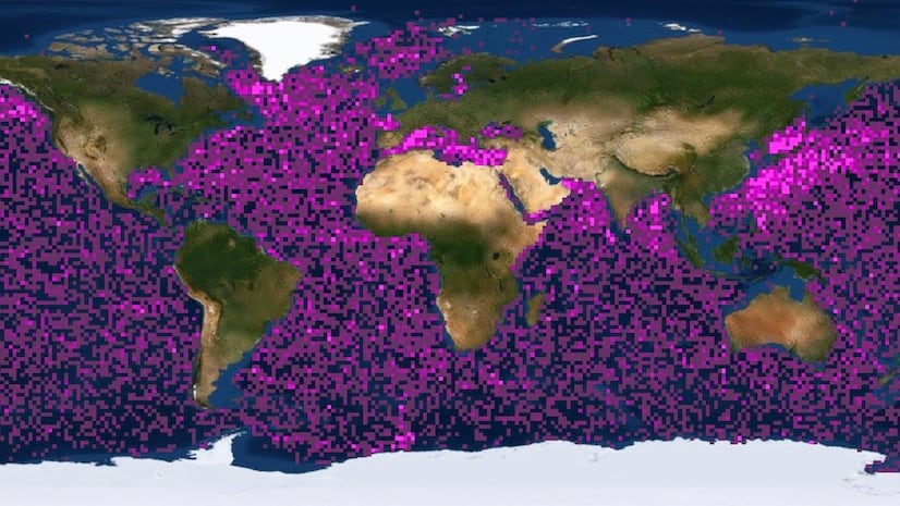
Argo float locations aggregated at a fixed bin level of 3. Level 3 is probably more useful at regional extents, but the global view can be a nice way to show density at a higher resolution. Binning allows you to see the density of features based on a geographic grid of cells.

What is binning?

Binning aggregates data to predefined cells, effectively representing point data as a gridded polygon layer. Typically, bins are styled with a continuous color ramp and labeled with the count of points contained by the bin. The JS API uses the public domain geohash geocoding system to create the bins.

This is an effective way to show the density of points. Unlike clustering, binning shows point density in geographic space, not screen space.

Binning allows you to effectively visualize where points stack on top of another or are in very close proximity to each other. Use the swipe widget above to compare a layer of points with a binned version of the same data.

Why is binning useful?

Large point layers can be deceptive. What appears to be just a few points can in reality be several thousand. Binning allows you to visually represent the density of points in a geographic grid of cells.

For example, the following map shows the locations of thousands of Argo floats (similar to a buoy). Regions A and B both have a high density of points, making them impossible to compare without additional help.

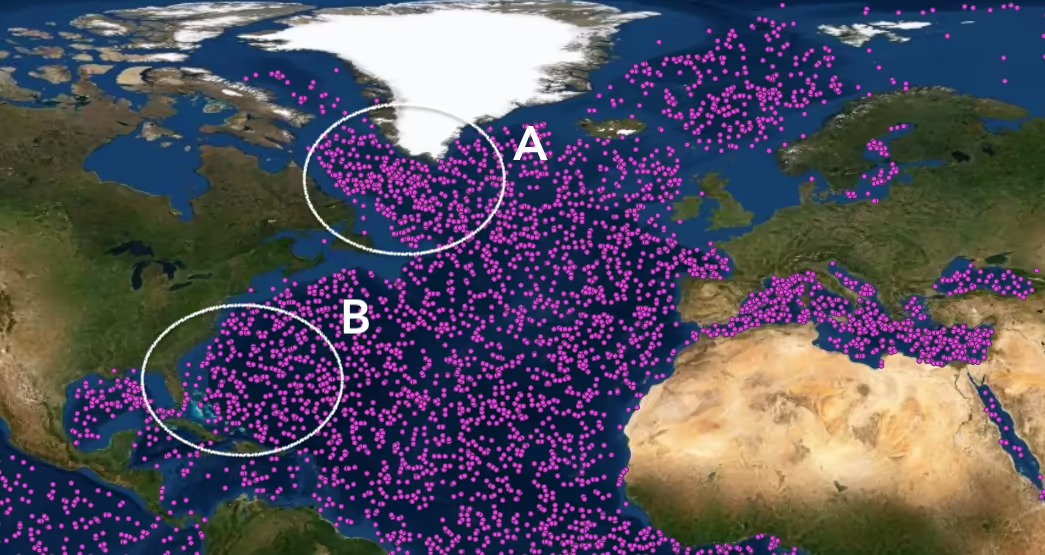
Region A and region B both have a high density of points. It is impossible to tell how many points overlap in each area.

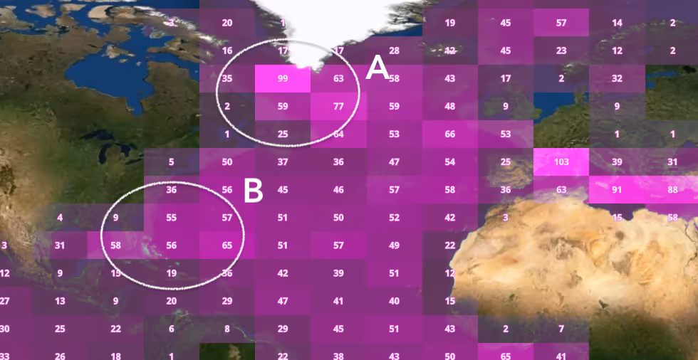
However, when binning is enabled, the user can now clearly compare the density of both regions.

Binning allows the user to easily compare the density of overlapping features at a glance.

How binning works

Binning is configured on the featureReduction property of the layer. You can enable binning with minimal code by setting the featureReduction type to binning.

Use dark colors for code blocksCopy
layer.featureReduction = {
  type: "binning"
};

Since binning does not have a default renderer, you won't be able to see the bins without explicitly defining a renderer. The featureReduction property gives you control over many other binning properties, including the following:

fixedBinLevel - Determines the resolution of the grid (only accepts values 1-9). Larger numbers result in a higher resolution. Low numbers result in a coarse resolution.
fields - Defines how to aggregate the layer's fields based on a statistic type.
renderer - Defines the style of the bins.
popupTemplate - Allows you to summarize data in the bin when the user clicks it.
labels - Typically used to label each bin with the number of points it represents.

Examples

Basic binning

The following example demonstrates how to enable binning on a point layer and configure the renderer, labels, and a popup for displaying the point count inside each bin. You must select a fixedBinLevel between 1-9 when enabling binning. Choose a bin level based on the data extent. The following table describes suggested bin levels given your data extent.

Fixed bin level	Suggested data extent
1-3	Global extents.
3-5	Regional extents (e.g. countries and states).
5-7	Local communities (e.g. counties and cities).
7-9	Hyper local areas (e.g. neighborhoods and buildings).

You must also define aggregate fields to make the binning visualization meaningful. An aggregate field determines how to represent data from the underlying layer in its aggregate form (i.e. the bin). For example, to create an aggregate field for point count inside the bin, use the count statistic type.

Use dark colors for code blocksCopy
layer.featureReduction = {
  type: "binning",
  fixedBinLevel: 2,
  fields: [{
    name: "aggregateCount",
    statisticType: "count"
  }]
};

This can now be used in the renderer, labels, and popup for each bin. These properties are configured just as they would be on any other layer type, except they must refer to aggregate fields defined in FeatureReductionBinning.fields instead of the underlying layer's fields. Typically, bins are styled with a continuous color visual variable as demonstrated in this example.

Argo float locations aggregated at a fixed bin level of 2. This is a great resolution for global data.

Expand
Use dark colors for code blocksCopy
        const featureReduction = {
          type: "binning",
          fixedBinLevel: 2,
          fields: [{
            name: "aggregateCount",
            alias: "Total count",
            statisticType: "count"
          }],
          renderer: {
            type: "simple",
            symbol: {
              type: "simple-fill",
              color: [0, 255, 71, 1],
              outline: null,
              outline: {
                color: colors[0],
                width: 0
              }
            },
            visualVariables: [
              {
                type: "color",
                field: "aggregateCount",
                legendOptions: {
                  title: "Number of floats"
                },
                stops: [
                  { value: 0, color: colors[0] },
                  { value: 25, color: colors[1] },
                  { value: 50, color: colors[2] },
                  { value: 75, color: colors[3] },
                  { value: 100, color: colors[4] }
                ]
              }
            ]
          },
Expand

Alternate binning styles

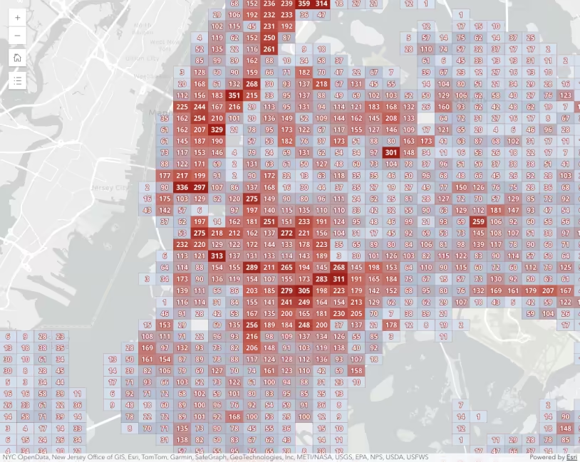
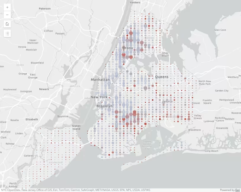
Bins can be styled with any renderer suitable for a polygon layer. This example demonstrates how to visualize bins based on two aggregate fields. The aggregate count is visualized with a size visual variable, and the average number of people injured in each crash is visualized using a color visual variable.

Car crashes (2020) aggregated to bins at a fixed level of 6. The size of each symbol indicates the total number of crashes. Color indicates the average number of injured motorists per crash.

Use dark colors for code blocks
Add line.Add line.Add line.Add line.Add line.Add line.Add line.Add line.Add line.Add line.        const featureReduction = {
          type: "binning",
          fixedBinLevel: 6,
          fields: [

            new AggregateField({
              name: "aggregateCount",
              statisticType: "count"
            }),
            new AggregateField({
              name: "AVG_MOTORIST_INJURED",
              alias: "Ratio of motorist injuries to crashes",
              onStatisticField: "NUMBER_OF_MOTORIST_INJURED",
              statisticType: "avg"
            }),

          ],
          renderer: {
            type: "simple",
            symbol: {
              type: "simple-marker",
              color: [0, 255, 71, 1],
              outline: null,
              outline: {
                color: "rgba(153, 31, 23, 0.3)",
                width: 0.3
              }
            },

            visualVariables: [
              {
                type: "size",
                field: "aggregateCount",
                legendOptions: {
                  title: "Total crashes"
                },
                minSize: {
                  type: "size",
                  valueExpression: "$view.scale",
                  stops: [
                    { value: 18055, size: 18 },
                    { value: 36111, size: 12 },
                    { value: 72223, size: 8 },
                    { value: 144447, size: 4 },
                    { value: 288895, size: 2 },
                    { value: 577790, size: 1 }
                  ]
                },
                maxSize: {
                  type: "size",
                  valueExpression: "$view.scale",
                  stops: [
                    { value: 18055, size: 48 },
                    { value: 36111, size: 32 },
                    { value: 72223, size: 24 },
                    { value: 144447, size: 18 },
                    { value: 288895, size: 12 },
                    { value: 577790, size: 6 }
                  ]
                },
                minDataValue: 10,
                maxDataValue: 300
              },
              {
                type: "color",
                field: "AVG_MOTORIST_INJURED",
                legendOptions: {
                  title: "% of motorists injured per crash"
                },
                stops: [
                  { value: 0, color: colors[0], label: "No injuries" },
                  { value: 0.1, color: colors[1] },
                  { value: 0.3, color: colors[2], label: "30%" },
                  { value: 0.5, color: colors[3] },
                  { value: 0.75, color: colors[4], label: ">75%" }
                ]
              }
            ]

          }
        };