1.1 Release notes

1.1.1 Patch Release notes

The 1.1.1 patch release of ArcGIS GeoAnalytics Engine adds support for Spark 3.3.2, Java 17 and fixes issues related to OAuth tokens, Group by Proximity relationships, time fields' return type, and writing to Feature Services.

1.1.0 Release notes

The 1.1.0 release of ArcGIS GeoAnalytics Engine adds a variety of new features including new SQL functions, analysis tools, spatial data sources, plotting capabilities, and utilities for exploring spatial references and transformations. This release also adds support for Spark 3.3.1 and the latest runtimes for Databricks and AWS EMR.

SQL functions

Version 1.1.0 adds 10 new SQL functions to GeoAnalytics Engine:

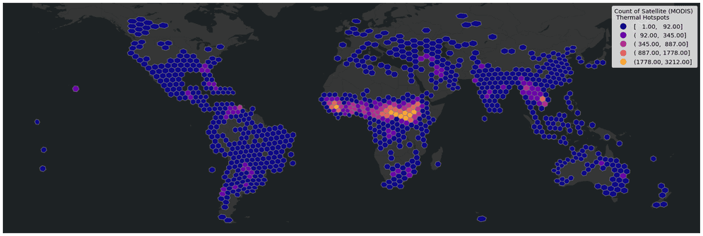
• ST_H3Bin and ST_H3Bins—Return the H3 bin or bins that intersect with a geometry. H3 is an open source, hierarchical geospatial indexing system that partitions the world sphere into hexagonal and pentagonal tiles. Like square or hex bins, H3 bins can be used to index, aggregate, and summarize data. For example, the plot below shows seven days of satellite-detected thermal hotspot points aggregated into H3 bins and colored using the count of points within each bin.

  

• ST_BinId—Takes a bin column and returns the ID of each bin as a long integer. Bin IDs can be used to persist bins in any file format. You can also now create bins from a bin ID. In the case of H3, the H3 bin ID can be used for interoperability with other systems that work with H3 indices.

• ST_Densify and ST_GeodesicDensify—Add vertices along geometries to create densified geometries where each segment is no longer than a specified maximum length.

• ST_ClosestPoint and ST_GeodesicClosestPoint— Take two geometries and return a point on the first geometry that is the closest to the second geometry.

• ST_ShortestLine and ST_GeodesicShortestLine— Take two geometries and return the shortest line that touches the two geometries.

• ST_SRText—Can get or set the spatial reference of a geometry column using the Well-Known Text (WKT) representation of the spatial reference.

Tools

GeoAnalyics Engine 1.1.0 includes two new analysis tools: Snap Tracks and Nearest Neighbors. The release also includes added support for performing a left one-to-many join in the Spatiotemporal Join tool.

Snap Tracks

Snap Tracks takes time-enabled points (e.g., GPS movement data with a timestamp) and snaps them to lines (e.g., roads or paths) so you can gain a clearer understanding of which lines the points traveled along.

To match the points to lines, the tool considers the distance between points and the candidate lines, as well as the points’ ability to move along the lines. That means, if your points are moving in one direction, they won’t snap to lines that only support movement in another direction. For example, say you are tracking a fleet of vehicles using GPS and want to know how much time each vehicle spent on each segment of road in an area. Using Snap Tracks, you can account for GPS error and quickly understand which road segment each GPS point should be on. The animation below shows GPS data before (in green) and after (in blue) being processed with Snap Tracks.

Nearest Neighbors

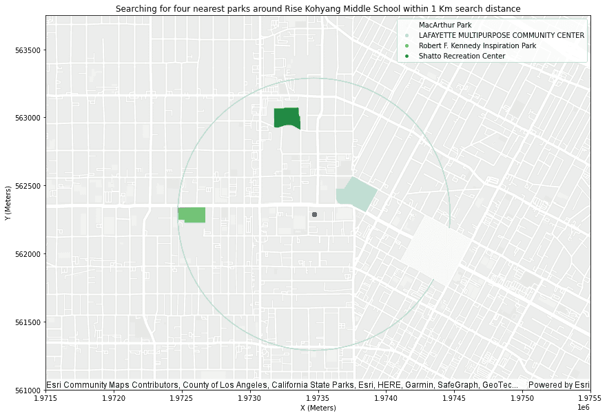
Nearest Neighbors finds the given number of neighbors to a record in a DataFrame from records in another DataFrame. The records from the input DataFrames are matched based on closest proximity. For example, say you want to enrich housing data with information about schools near each home. With a point dataset representing schools and a polygon dataset representing homes, you could use the Nearest Neighbors tool to find the 5 closest schools to each home and enrich the homes data with statistics about the schools. This could be used for visualization or further analysis.

Left Join

With the 1.1.0 release, the Spatiotemporal Join tool now supports a left one-to-many join where all input records will be included in the result DataFrame without requiring summarization of the joined records. You can also utilize an optimized spatial join with pyspark.sql.DataFrame.join when joining on the result of a ST function from GeoAnalytics Engine. This is supported for inner, left and left_outer joins.

Visualization

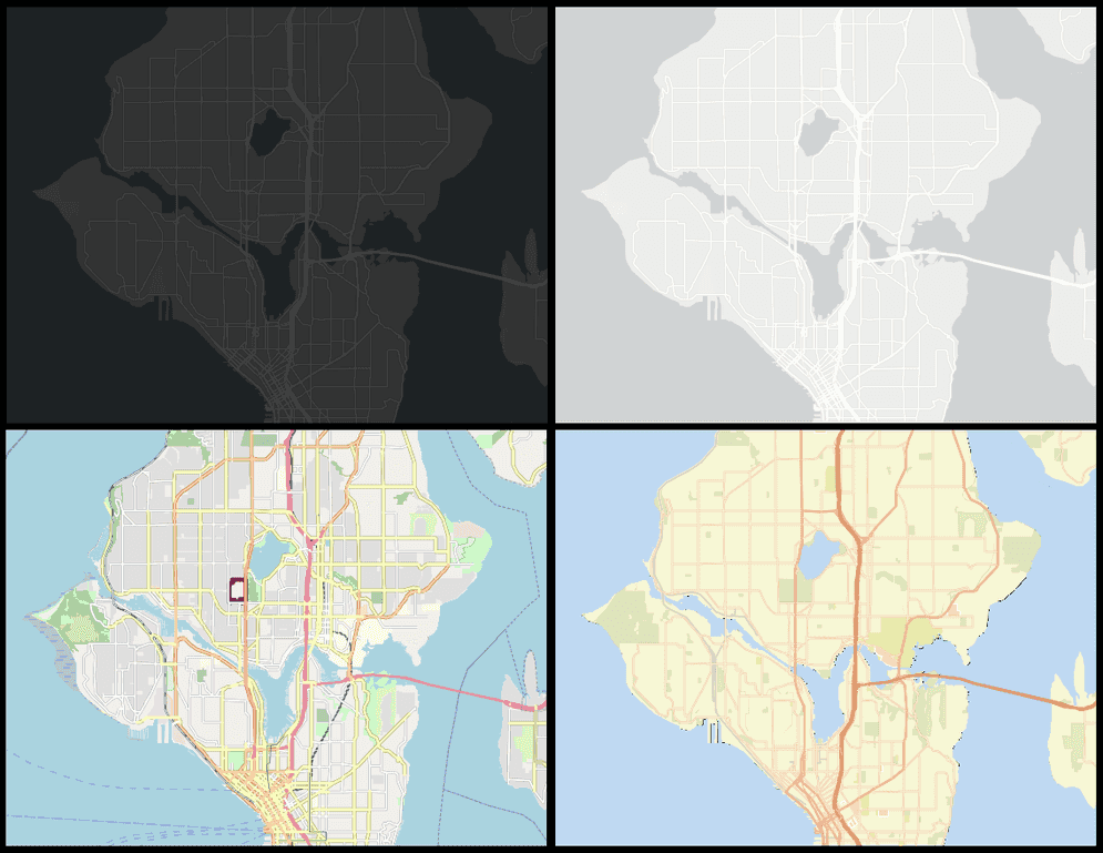
The plotting method included with GeoAnalytics Engine now includes support for plotting basemaps, so you can quickly gain geographic context when viewing your geometry data. The plots below show four examples of basemaps available in version 1.1.0. For more information, see the core topic for Visualizing results and the tutorial for Visualizing results with st.plot().

Data sources

You can now read from and write to GeoJSON and GeoParquet files using GeoAnalytics Engine. When reading from or writing to these formats, GeoAnalytics Engine will automatically handle any geometry data and its associated metadata, allowing for easy interoperability with other systems that work with these formats.

GeoAnalytics Engine 1.1.0 also adds support for writing feature services to ArcGIS Online or ArcGIS Enterprise. After connecting to ArcGIS Online or ArcGIS Enterprise with the new register_gis function, you can either save a DataFrame as a new feature service, append to an existing feature service layer, or create a new feature layer in an existing feature service. Registering a GIS also allows you to read data from a secured feature service layer in ArcGIS Enterprise or ArGIS Online. For examples, see the tutorials on Write to feature services and Read from feature services.

Utilities

Version 1.1.0 adds several utilities related to coordinate systems and transformations. These functions help you discover the best spatial reference to use, search for specific transformations, and validate your data.

• create_optimal_sr—Creates a spatial reference with a custom projected coordinate system optimal for the data extent and intended purpose of your analysis. The function returns a SpatialReference object which can be passed to ST_Transform to transform your geometry data to a spatial reference suited best to your objectives.

• list_transformations—Returns a DataFrame with a list of valid transformation methods between two spatial references and for a given extent. This list can help you decide which transformation to use when transforming your geometry data. Also new in version 1.1.0, you can explore the transformations and spatial references available in GeoAnalytics Engine using Spark SQL, as shown below.

  Use dark colors for code blocksCopy

  1
  2
  spark.sql("SELECT Name, Code, FromCode, ToCode, AreaOfUse " + \
            "FROM geoanalytics.system.transformations").show(5, truncate=False)
  Use dark colors for code blocksCopy

  1
  2
  3
  4
  5
  6
  7
  8
  9
  10
  +------------------------+----+--------+------+----------------------------+
  |Name                    |Code|FromCode|ToCode|AreaOfUse                   |
  +------------------------+----+--------+------+----------------------------+
  |MGI_To_ETRS_1989_4      |1024|4312    |4258  |\{13.58, 46.64, 16.17, 47.84\}|
  |Ain_el_Abd_To_WGS_1984_3|1055|4204    |4326  |\{46.54, 28.53, 48.48, 30.09\}|
  |Ain_El_Abd_To_WGS_1984_4|1056|4204    |4326  |\{46.54, 28.53, 48.48, 30.09\}|
  |Ain_El_Abd_To_WGS_1984_5|1057|4204    |4326  |\{46.54, 29.1, 48.42, 30.09\} |
  |Ain_El_Abd_To_WGS_1984_6|1058|4204    |4326  |\{46.54, 28.53, 48.48, 29.45\}|
  +------------------------+----+--------+------+----------------------------+
  only showing top 5 rows
  Use dark colors for code blocksCopy

  1
  2
  spark.sql("SELECT Code, Name, Type, Units, Tolerance, AreaOfUse " + \
            "FROM geoanalytics.system.spatial_references").show(5, truncate=False)
  Use dark colors for code blocksCopy

  1
  2
  3
  4
  5
  6
  7
  8
  9
  10
  +----+------------+----------+------+--------------------+------------------------------+
  |Code|Name        |Type      |Units |Tolerance           |AreaOfUse                     |
  +----+------------+----------+------+--------------------+------------------------------+
  |3819|GCS_HD1909  |Geographic|Degree|8.984194981201908E-9|\{16.11, 45.74, 22.9, 48.58\}   |
  |3821|GCS_TWD_1967|Geographic|Degree|8.983120447446023E-9|\{119.25, 21.87, 122.06, 25.34\}|
  |3824|GCS_TWD_1997|Geographic|Degree|8.983152841195215E-9|\{114.32, 17.36, 123.61, 26.96\}|
  |3889|GCS_IGRS    |Geographic|Degree|8.983152841195215E-9|\{38.79, 29.06, 48.75, 37.39\}  |
  |3906|GCS_MGI_1901|Geographic|Degree|8.984194981201908E-9|\{13.38, 40.85, 23.04, 46.88\}  |
  +----+------------+----------+------+--------------------+------------------------------+
  only showing top 5 rows

• set_spatial_reference—Sets the spatial reference of a geometry column in a DataFrame, an alternative to using ST_SRID.

• get_extent—Returns a BoundingBox object representing the spatial extent of the geometries in a geometry column. This is a straightforward way to verify that your geometry data is located where you would expect it to be. A BoundingBox can can also be passed to create_optimal_sr or list_transformations as the extent parameter to easily limit the spatial reference or transfomation search to only what matters to your data. Similarly, you can use it when plotting to quickly set the visual extent of your plot or to filter your data prior to plotting.

In addition to the new functions and utilities listed above, the supplemental projection and transformation data included with GeoAnalytics Engine has been updated to include the latest NADCON and NADCON5 transformation data as well as new NTV2 data for transformations in Australia, Canada, Iceland, the Netherlands, and the UK.

Spark 3.3 and new cloud runtime support

With every release, support for the latest Spark versions and cloud runtimes are added if possible. In 1.1.0, GeoAnalytics Engine adds support for Spark 3.3.1 and the latest of the following cloud runtimes:

• Databricks (11.3 LTS, 12.0, 12.1)
• AWS EMR (6.8.x, 6.9.x)

Additional documentation

The new Data Sources section in the GeoAnalytics Engine guide was added to provide guidance for bringing your big data into Spark through data sources included with Spark like CSVs, Parquet, and ORC. It also includes documentation for data sources included with GeoAnalytics Engine such as Shapefile, Feature Service, and now GeoJSON and GeoParquet.

Also, the GeoAnalytics Engine install guide now includes documentation for Databricks on AWS in addition to Azure Databricks.