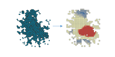
Given a DataFrame, Find Hot Spots identifies statistically significant hot spots and cold spots using the Getis-Ord Gi* statistic.
Usage notes
-
Find Hot Spots identifies statistically significant spatial clusters of many records (hot spots) and few records (cold spots). It creates an output DataFrame with a z-score, p-value, and confidence level bin (Gi_Bin) for each binned area.
-
During analysis, the input points (incidents) are aggregated into bins of a specified size, and are then analyzed to determine hot spots. The aggregated bins must contain a variety of values (counts of points in a bin should be highly variable).
-
The z-scores and p-values are measures of statistical significance that tell you whether to reject the null hypothesis using aggregated bins. That is, they indicate whether the observed spatial clustering of high or low values is more pronounced than one would expect in a random distribution of those values. The z-score and p-value fields do not reflect any kind of False Discovery Rate (FDR) correction.
-
The
Gifield identifies statistically significant hot and cold spots. Records in the +/-3 bins reflect statistical significance with a 99 percent confidence level; records in the +/-2 bins reflect a 95 percent confidence level; records in the +/-1 bins reflect a 90 percent confidence level; and the clustering for records in bin 0 is not statistically significant.Bin -
A high z-score and small p-value for an input row indicates an intense presence of point incidents. A low negative z-score and small p-value indicates an absence of point incidents. The higher (or lower) the z-score, the more intense the clustering. A z-score near zero indicates no apparent spatial clustering.
-
The z-score is based on the randomization null hypothesis computation.
-
Find Hot Spots requires that your input DataFrame's geometry has a projected coordinate system. If your data is not in a projected coordinate system, the tool will transform your input to a World Cylindrical Equal Area (SRID: 54034) projection. You can transform your data to a projected coordinate system by using ST_Transform.
-
You can optionally use
setto find hot spots within time steps. This setter can only be used if the input points are time enabled and represent an instant in time. TheTime Step() alignmentparameter specifies how time steps will be aligned and can be one of the following:End—Time steps will align to the last time event and aggregate back in time. This is the default.Time Start—Time steps will align to the first time event and aggregate forward in time.Time Reference—Time steps will align to the date or time specified byTime reference._time
-
When input records are analyzed using time steps, each time step is analyzed independent of records outside of the time step.
-
The bin size specifies the area that points will be aggregated into for analysis. The neighborhood is the spatial extent of the analysis. This value determines which bins are analyzed together in order to assess local clustering.
Limitations
-
The input must be a DataFrame with point geometries, and they will be aggregated into bins of a specified size before analysis.
-
You cannot find hot spots based on a field value.
-
Setting the time step repeat interval is not supported. Hot spots can only be found within continuous time step intervals.
Results
The output includes records representing bins with the following new fields:
| Field | Description |
|---|---|
| datetime | If your input had a timestamp column and used time stepping, the output will have a start time column, step, and an end time column, step, to represent the time step interval. |
bin | The polygonal bins. |
value | The count of records in the given bin named geometry is created that represents polygonal bins. |
Gi | The z-score. |
Gi | The p-value. |
Gi | Bins of +-0, 1, 2 representing the statistical significance confidence level. |
Performance notes
Improve the performance of Find Hot Spots by doing one or more of the following:
-
Only analyze the records in your area of interest. You can pick the records of interest by using one of the following SQL functions:
- ST_Intersection—Clip to an area of interest represented by a polygon. This will modify your input records.
- ST_BboxIntersects—Select records that intersect an envelope.
- ST_EnvIntersects—Select records having an evelope that intersects the envelope of another geometry.
- ST_Intersects—Select records that intersect another dataset or area of intersect represented by a polygon.
- Create larger bins and a smaller neighborhood.
Similar capabilities
Similar tools:
How Find Hot Spots works
Even random spatial patterns exhibit some degree of clustering. In addition, our eyes and brains naturally try to find patterns even when none exist. Consequently, it can be difficult to know if the patterns in your data are the result of real spatial processes at work or just the result of random chance. This is why researchers and analysts use statistical methods like Find Hot Spots (Getis-Ord Gi*) to quantify spatial patterns.
For point data that represents an event, incident, or indication of presence or absence, you just want to know where clustering is unusually (statistically significant) intense or sparse. For this analysis, areas (a grid of bins that the tool creates for you) are placed over the points, and the number of points that fall within each area are counted. The tool then finds clusters of high and low point counts associated with each area. The tool calculates the Getis-Ord Gi* statistic (pronounced "G-i-star") for each binned area in a DataFrame. The resultant z-scores and p-values tell you where areas with either high or low values cluster spatially.
Each area is analyzed within the context of neighboring areas. An area with a high value is interesting, but it may not be a statistically significant hot spot. To be a statistically significant hot spot, an area will have a high value and also be surrounded by other areas with high values. The local sum for an area and its neighbors is compared proportionally to the sum of all areas; when the local sum is very different from the expected local sum, and when that difference is too large to be the result of random chance, a statistically significant z-score results.
When you do find statistically significant clustering in your data, you have valuable information. Knowing where and when clustering occurs can provide important clues about the processes driving the patterns you're seeing. For example, finding statistically significant spatial clustering of cancer associated with certain environmental toxins can lead to policies and actions designed to protect people. Similarly, finding cold spots of childhood obesity associated with schools promoting after-school sports programs can provide strong justification for encouraging these types of programs more broadly.
Syntax
For more details, go to the GeoAnalytics Engine API reference for find hot spots.
| Setter (Python) | Setter (Scala) | Description | Required |
|---|---|---|---|
run(dataframe) | run(input) | Runs the Find Hot Spots tool using the provided DataFrame. | Yes |
set | set | Sets the size of square bins used to find hot spots. | Yes |
set | set | Sets the size of the neighborhood used to find hot spots. | Yes |
set | set | Sets the time step interval duration and the time step interval alignment. If set, hot spots will be calculated for each time step at each bin location. | No |
Examples
Run Find Hot Spots
# Imports
from geoanalytics.tools import FindHotSpots
from geoanalytics.sql import functions as ST
# Path to the earthquakes data
data_path = r"https://sampleserver6.arcgisonline.com/arcgis/rest/services/" \
"Earthquakes_Since1970/FeatureServer/0"
# Create an earthquakes DataFrame and transform the geometry to World Cylindrical Equal Area
df = spark.read.format("feature-service").load(data_path) \
.withColumn("shape", ST.transform("shape", 54034))
# Use Find Hot Spots to uncover global earthquake hot spots
result = FindHotSpots() \
.setBins(bin_size=250, bin_size_unit="Miles") \
.setNeighborhood(distance=500, distance_unit="Miles") \
.run(dataframe=df)
# Show the first 5 rows of the result sorted by Gi_Bin column values
result.sort("Gi_Bin", ascending=False).show(5)+-----+------------------+--------------------+------+--------------------+
|value| GiZScore| GiPValue|Gi_Bin| bin_geometry|
+-----+------------------+--------------------+------+--------------------+
| 5.0|3.7607595687467907|1.693981921161063...| 3.0|{"rings":[[[15601...|
| 17.0| 3.83909573966328|1.234882743127410...| 3.0|{"rings":[[[23648...|
| 6.0| 2.66405317591594|0.007720535726935918| 3.0|{"rings":[[[15601...|
| 9.0| 3.785564505436045|1.533600453779985...| 3.0|{"rings":[[[19624...|
| 19.0| 4.102294557788669|4.090730293773235...| 3.0|{"rings":[[[19624...|
+-----+------------------+--------------------+------+--------------------+
only showing top 5 rowsPlot results
# Create a continents DataFrame and transform the geometry to World Cylindrical Equal Area
continents_path = "https://services.arcgis.com/P3ePLMYs2RVChkJx/ArcGIS/rest/" \
"services/World_Continents/FeatureServer/0"
continents_df = spark.read.format("feature-service").load(continents_path) \
.withColumn("shape", ST.transform("shape", 54034))
# Plot the resulting earthquake hot spots
continents_plot = continents_df.st.plot(facecolor="none",
edgecolors="lightblue",
figsize=(16,12),
basemap="light")
result_plot = result.st.plot(cmap_values="Gi_Bin",
cmap="Wistia",
legend=True,
legend_kwds={"orientation": "vertical", "location": "right", "shrink": 0.3, "pad": 0.05},
ax=continents_plot)
result_plot.set_title("World earthquake hot spots")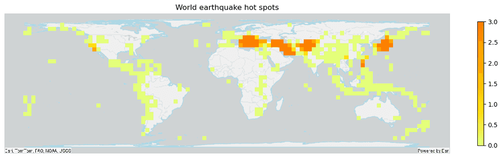
Version table
| Release | Notes |
|---|---|
1.0.0 | Python tool introduced |
1.6.0 | Scala tool introduced |